This failure among others has led many to view nominal GDP as the new target of choice. But as we have this new conversation, we should not forget about how to change our approach to the instrument. In particular, to what extent does the Taylor Rule still matter? In this post, I will argue that the Taylor Rule can actually be a powerful template for better policy. By modifying the Taylor Rule to be sensitive to the absolute level of the interest rate, the Fed would have a flexible yet robust policy regime that effectively harness the most important tool of monetary policy: expectations.
Section 1 reviews the concept of the Taylor Rule, Section 2 discusses the modification, Section 3 compares the new rule with the historical data, Section 4 connects the new rule to other policy proposals, and Section 5 concludes.
1. Introduction
The principle behind the Taylor rule is to adjust the short term interest rate based on inflation and the output gap. The original rule from John Taylor's 1993 article is:

Where r is the short term nominal interest rate, π is the rate of inflation over the past year, and y is the percent deviation of real GDP from its trend. From a positive perspective, this simple rule fits past Fed policy quite well. From a normative perspective, its clear description of what monetary policy was during the good times can hopefully give us better guidance on what monetary policy should be during the bad.
The Taylor Rule, because it is so simple, also helps with setting a rule-based policy. There is a long literature on the differences between discretionary and systematic policy, and the general conclusion is that systematic policy, because it can shape expectations of future inflation, is more effective at stabilizing the economy. The Taylor Rule is systematic because it is a transparent rule. This allows the central bank to shape expectations of how the Fed will act. As a result, the central bank provides markets with more certainty over the future path of economic growth.
While the coefficients are merely rules of thumb, one important note is that the coefficient on inflation should be greater than 1. This is known as the Taylor Principle. It is because real, not nominal, interest rates drive inflation. Therefore, the nominal interest rate needs to rise by more than 1% for every 1% increase in inflation to stabilize inflation. This is a good rule for most times, although down below I will argue that there are better options for low interest rate environments.
2. A Rate Dependent Taylor Rule
2.1 Motivation
A limitation of the traditional Taylor Rule is that the coefficients are constant across all values of the interest rate, inflation, and the output gap. However, the relative costs of inflation and output gaps change depending on the interest rate. When interest rates are very low, inflation has the collateral benefit of helping the central bank avoid (potentially self-imposed) policy difficulties at the zero lower bound. On the other hand, if interest rates are already very high, excessive inflation merely adds to economic uncertainty.
Therefore, the weights on the Taylor Rule should not be identical in all states of nature. Rather, because the relative costs of inflation and output gaps change depending on the interest rate, the Taylor Rule coefficients should also adjust.
This makes debates over particular coefficients quite silly. Instead of arguing over whether the output gap should have a coefficient of 0.5 or 1, the question should be how to systematically adjust those coefficients.
For example, when Nikolsko-Rzhevskyy and Papell evaluate whether Taylor Rules should justify Quantitative Easing, they conclude that a proper Taylor Rule would not. Although a Taylor Rule that heavily weights the output gap may justify QE, they argue the rule should be rejected because it would not have been hawkish enough on inflation in the 1970's. However, this implicitly assumes that policy makers cannot vary their weights on output and inflation over time. But if these changing weights can be specified in a transparent rule, then it's very likely that the optimal rule would involve both strict tightening in the 1970's and aggressive easing right now.
2.2 Specification
With the traditional rule in mind, I now propose an alternative that I call the Rate Dependent Taylor Rule. In this rule, set the instantaneous target (v) at

For some functions f and g that are weakly increasing and decreasing in the interest rate, respectively. Then set the actual rate as a weighted average of the interest rate last period and the current instantaneous target

Therefore, a particular specification could be:
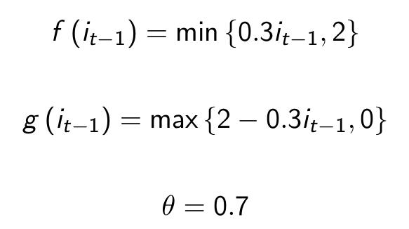
These response coefficients are plotted in the following chart. Observe that at the black line when the interest rate is 5, the two Rate Dependent coefficients match the traditional Taylor Rule.

There are three key design features of this specification.
First, the values of these coefficients are fixed in the range between 0 and 2. The logic behind this is to prevent excessive volatility in the interest rate. With these bounds, we also have justification for the slopes of 0.3. Recall that for the original rule, the coefficient on inflation was fixed at 1.5 and the coefficient on the output gap was fixed at 0.5. The modified rule takes on these values only if the interest rate is 5, the historical average of the federal funds rate. Therefore, the modified rule can both be more hawkish and more dovish than the original Taylor rule, contingent on economic conditions. This way, the modified Taylor rule can emulate the magnitude and volatility of the old Taylor rule, but also provide additional flexibility.
Second, when the interest rate is below 3.3, the example above actually violates the Taylor principle. This is no accident. Recall that the logic of the Taylor principle was to allow the central bank to keep a lid on inflation by ensuring that the real rate rises in response to inflation. But if interest rates are already at the low level of 2%, we actually want to encourage inflation so that the nominal rate can stay at the 5% level. Intuitively, this strengthens the negative feedback loop that keeps the nominal interest rate around 5%, giving the central bank more room to operate.
On one hand, excessive interest rate volatility can itself be harmful as agents spend more resources trying to avoid holding money. This is the argument for a Friedman rule for zero nominal interest rates, and although the argument is not as strong in the case, the logic still applies. High nominal rates can be distortionary, and thus their variance should be limited.
Moreover, without persistence it is hard for central banks to signal commitment to future interest rate paths. Future policy would be more unpredictable. Because the rate can change dramatically in response to new conditions, the Fed would not have a framework for commitment. Because one of the key selling points of a Taylor rule is to help guide expectations, to have an instrument that responds too quickly to economic conditions weakens the expectations channel. Therefore, the instrument should be persistent. In my rule, I choose a value of 0.7, which is very close to the value of 0.65 cited by Woodford.
3. Historical Comparisons
This specification is first compared against the traditional Taylor Rule and actual federal funds rate during the Great Moderation and up to the current period. Note that this isn't really a policy simulation. In fact the parameters that are rate dependent look at the actual federal funds rate in the previous period, not the rate-dependent rate. Therefore, this version gives a better picture of how the policy would give advice at each moment in time. In the future, I intend to further investigate the dynamics.

The bottom panel shows a running time series with the coefficients in front of inflation (blue) and output gaps (magenta) changing over time. This shows that although the traditional Taylor Rule matches the policy advice of the Rate Dependent rule for the second half of the 1990's, in general they do not always correspond.
Another historical period of interest is the 1970's and 80's. In this time, inflation was far too high. Therefore, an effective rule should call for more hawkish policy. Indeed, the Rate Dependent rule does that. It would have called for interest rates in the 1970's and 1980's to be up to 10 percentage points higher than they actually were, and approximately five percent higher than what the traditional Taylor rule would have called for.
This is similar to what Evan Soltas noted about how a nominal GDP target would have called for tighter policy in the 70's. Even though the Rate Dependent rule would at times call for easier policy to stabilize output, it is very hawkish when inflation is high. As such, it would still anchor inflation expectations with the promise of disciplined policy when inflation and the Fischer effect push up interest rates in the future.

4. Relationship with Forward Guidance, Nominal GDP Targeting, and a Virtual Fed Funds Rate
Although the Rate Dependent rule fits the historical data quite well, there is one large deviation. In the current environment, the rule says that the Fed should be easing. Hard. While the zero lower bound constrains the Fed from actually hitting the rate advocated by this rule, this does not mean the rule cannot help guide policy. In fact, the greatest appeal of the Rate Dependent rule at the current juncture would be its justification for forward guidance. If the large gap can't be closed with current short term rates, then perhaps it can be filled with future ones.
A Rate Dependent rule frames the current tightness in monetary policy by identifying a large deviations from a rule that fits the historical data. While this method may not be ideal, it shows how even the traditional framework of seeing monetary policy through instrument rules justifies aggressive easing at this juncture.
Moreover, the theoretical reasoning behind the Rate Dependent rule is much more familiar for those who think in terms of Taylor Rules. Unlike a nominal aggregate target, the Rate Dependent rule is a concrete policy that can be implemented. It helps to assuage the concerns of John Taylor when he complains that an open ended nominal GDP target fails to give "quantitative operational guidance about what the central bank should do with the instruments." This way, the Rate Dependent rule helps to justify additional easing to a broader audience.
This alternate framing also gets around potential credibility issues nominal GDP targeting. This is not to say a nominal GDP target would not be desirable but a 2012 Dallas Fed paper did bring up some credibility issues with such a target. Evan Koenig, the vice president of the Dallas Fed, pointed out that the Fed does not have a good record of stabilizing nominal GDP growth. A graph from the paper is reproduced below.

However, the historical comparisons above clearly show that the Rate Dependent rule is a good description of historical policy. Moreover the scatter plot below clearly shows that the Rate Dependent rule is also a good predictor of what a nominal GDP target would require. Therefore, the Fed can point to this rule and do a monetary two-step. While the Fed foxtrots into a more enlightened nominal GDP target, it can still maintain and demonstrate its credibility to this new policy path by justifying it with the historical experience.

The Rate Dependent rule is also a close cousin of the virtual Federal Funds rate, as advocated by my colleague Miles Kimball. In fact, the two proposals complement each other since the Rate Dependent rule provides a systematic approach for determining the virtual rate. This way, the Fed doesn't just ease when it "feels that monetary policy should be more expansionary." It would ease when it could point to the rule and say that it must.
5. Concluding Remarks
Of course, there is much work yet to be done. The above analysis is very descriptive and requires more formal modeling. In an upcoming post, I intend to discuss more about dynamics and the persistence of this rule. Doing more case study analyses of the rule in historical contexts would also be useful.
Much of the recent push for nominal GDP targets has neglected rules for the instrument. This omission runs the danger of confusion over the steps that need to be taken when a "whatever it takes" policy is declared. The Rate Dependent rule cuts through that confusion. It combines the rule based approach characteristic of traditional Taylor Rules with the recognition that the costs of inflation or output gaps can depend on the interest rate. In bridging various intellectual cousins, this policy forms a stronger basis for monetary easing now, while also committing to smart hawkishness later.

