Why Monetary Policy Should Ignore Financial Stability

Financial stability is apparently the new hot reason to tighten monetary policy, and in this article for Quartz I go in on some reasons for why this is a horrible idea. An excerpt

Janet Yellen’s confirmation hearing showed signs that US monetary policy will soon adopt a third mandate. She said: “Overall, the Federal Reserve has sharpened its focus on financial stability and is taking that goal into consideration when carrying out its responsibilities for monetary policy.” While Yellen has traditionally downplayed this mission, the December FOMC meeting minutes also revealed a growing chorus of FOMC participants who believe that monetary policy should do more than just ensure full employment and price stability. Rather, they believe that monetary policy should look out for bubbles and pop them before they jeopardize financial stability. 

At first glance, this sounds like a good idea. After all, who wants financial instability? 

But back in 2002, Bernanke outlined several reasons why tightening monetary policy in response to bubbles is unlikely to work in practice. First, there’s no reason to believe that the Fed can accurately identify bubbles in advance. Second, even if a bubble appears, it’s not clear that raising short term interest rates could pop it. Third, even if monetary policy ends up bringing asset prices down, it is likely to do so only through hurting the livelihoods of average Americans.

Something that should be added, though, is that I still believe research on how monetary policy affects financial stability can be useful. Such research can help us better understand how monetary policy transmission might work, and what things regulators should look out for as the monetary policy landscape changes. However, none of this is any reason why the central bank should base the stock of money on the caprices of the financial markets.

A Reply to Steve Williamson -- Why Dynamic Stories are Important

Steve Williamson caused a firestorm in the blogosphere over his modeling results that helicopter drops in liquidity traps reduce the inflation rate. While hist first few posts were filled with mathematical equations, he was gracious enough in a recent post to present a story of what's going on in the model (my emphasis is bolded)

Next, conduct a thought experiment. What happens if there is an increase in the aggregate stock of liquid assets, say because the Treasury issues more debt? This will in general reduce liquidity premia on all assets, including money and short term debt. But we're in a liquidity trap, and the rates of return on money and short-term government debt are both minus the rate of inflation. Since the liquidity payoffs on money and short-term government debt have gone down, in order to induce asset-holders to hold the money and the short-term government debt, the rates of return on money and short-term government debt must go up. That is, the inflation rate must go down. Going in the other direction, a reduction in the aggregate stock of liquid assets makes the inflation rate go up.

Translated further, Steve's story is as follows:

1. The central bank prints more money
2. People don't want to hold onto that money
3. To make sure people hold onto that money, the inflation rate must fall (to make holding money more attractive)
4. Hence, printing money lowers the inflation rate.

Any cursory scholar of monetary economics should find that counterintuitive. I would suggest that it's counterintuitive because it's, well, wrong. In particular, the jump from (2) to (3) isn't clear at all. If everybody receives a helicopter drop, and nobody wants to spend it, then how does inflation fall? Or in the words of Paul Krugman: "How does this requirement translate into an incentive for producers of goods and services — remember, we’re talking about stuff going on in the real economy — to raise prices less or cut them?"

On the other hand, a much more realistic view would be a "monetary disequilibrium" or otherwise stated as David Hume's price specie flow mechanism as described by David Hume in his essay "On Money". At the moment that people get more money, the inflation rate is fixed. Hence the rate of return isn't high enough to hold money, and so people spend that money. This causes prices to rise and generates inflation.

Here's the fundamental problem with Steve's model: he acts as if equilibrium conditions are enough to explain causality. Sure, in equilibrium it must be that the inflation rate must equal the liquidity value of holding onto money. But that can happen in two ways. Either the inflation rate could fall (Steve's story), or people could hold less cash lower real cash balances, thereby raising the marginal value of their liquidity holdings. Dynamic stories matter, and if you can't explain how you get to equilibrium, you may end up on the wrong side of truth.

Edit: Adjusted for a few comments from Nick Rowe

Quartz: Emerging markets need to stop focusing on their exchange rates

Here's a link to my 3rd Quartz article on how much of the emerging market sell-off was about monetary policy failures in the emerging markets themselves. In particular, by trying to maintain exchange rate policies, central banks in these countries overexpose themselves to foreign economic conditions. The highly positive response to the recent delay of taper serves as further evidence that many of these emerging economies need better ways of insulating themselves from foreign monetary shocks. Much of the work, draws on blog posts from Lars Christensen. His examples comparing monetary policy in Australia and South Africa versus policy in Brazil and Indonesia were particularly helpful. A few excerpts:

The sell-off in emerging markets is not an omen of a prolonged economic contraction. Although capital flows were also turbulent after the 2008 financial crisis, growth in emerging markets continued. Nor is this a sign of financial crisis. “One thing most people seem to agree on is that this is not a replay of the late 1990s,” writes Ryan Avent in the Economist. A combination of exchange rate flexibility and low external debt means that emerging markets are unlikely to experience the same level of carnage as was seen in the 1997. Rather, the sell-off is a statement about how monetary policy has been unable to stabilize output in emerging markets and the importance of monetary reform. 

...Since all capital controls eventually leak, emerging markets can commit to stabilizing either the exchange rate or domestic output—not both. Economists Joshua Aizenman, Menzie Chinn, and Hiro Ito (pdf) have shown that this tradeoff is real. In the 1972 to 2006 time period, “Greater monetary independence [was] associated with lower output volatility while greater exchange rate stability [implied] greater output volatility.” 

Between these two options, the answer should be clear. Central banks in emerging markets need to focus on domestic output, and not the exchange rate.

A Primer On General Equilibrium, or Why Money Matters

This post is meant to be a short summary of how to think about macroeconomics in terms of general equilibrium. During my conversations with Michael Darda this past summer, it became painfully apparent that clients tend to struggle with how to put money and goods markets together. As a result, I thought I should put together a little piece on my basic approach to thinking through these kinds of "across market" effects, and why it matters for some of the policy debates of our day.

Any macroeconomy can be broken down into two main markets: a real market for current goods and services, and a financial market for claims on future goods and services. For brevity, I will reduce the model for financial assets to the market for money, which, because of money's role as a store of value and medium of exchange, captures the notion of "claims on goods". To simplify further, I take all the markets for goods and reduce them down to one composite market, say, for apples. From this caricature, we can start thinking about how markets fit together.

In normal times, people receive apples and money from the sky in the form of endowments (i.e. their wealth), and they make decisions about how to balance their cash and apple balances. Apples are transacted, bellies are filled, and life is good.

But suddenly, a recession hits. What does this look like? By definition, a recession is when there is a general glut of goods that aren't consumed. In this toy economy, this corresponds to a situation in which some people have apples but choose not to eat them! This may seem peculiar, but remember that the market for apples in this model represents a composite of all goods markets. So it could be the case that while everybody has apples, some want Red Delicious while others are looking for the tartness of Granny Smith. In more formal economic models, this is glibly incorporated by requiring that people do not consume their own endowment and instead trade for consumption. In any case, apples aren't eaten and we have a rotten general glut.

But this seems peculiar -- aren't markets supposed to clear? Not necessarily. Prices don't always adjust instantly, so we can have excess supplies and excess demands. However, economists do have a way to constrain what this non-clearing state looks like. In particular, according to Walras' law, assuming everybody spends all of their wealth, if there are excess supplies (i.e. too much produced) in some markets, then they must add up to excess demands (i.e. too little produced) in other markets. In other words, even if supply does not equal demand in each market, supplies must add up to demands across markets.

The requirement that everybody spends their endowment is crucial. It means that Walras' law doesn't apply just to the market for apples because not everybody spends all their wealth on apples. Instead, some people may put their wealth in money. But once we include the money market, we do have the condition that everybody spends their endowment, and therefore Walras' law does apply to the entire macroeconomy of apples and money.

This leads to the most important conclusion from general equilibrium theory as related to monetary economics:

If there is an excess supply of goods, it must be the result of excess demand for money.

The goods market by itself is not enough to generate a recession with a general glut of goods. Only when there is the possibility of excess demand in money markets can recessions actually occur. Therefore the market for money is what gives a macroeconomy its business cycle feel. This is why money is so important for macro -- fluctuations in the money market are the proximate cause for any general fluctuation in the goods market. This is why, as Miles Kimball says, money is the "deep magic" of macro.

While this "apples and money" approach is the canonical presentation of general equilibrium, it is not the unique representation. For another interpretation, think about what the financial market really is. Since it represents the entire universe of claims on future goods, finance can be understood as a veil between the present and the future. So instead of focusing on the relationship between goods and financial markets at one point in time, we can cut out the middle man and instead think of general equilibrium as a sequence of goods markets that occur across multiple points in time. In this version, there is no financial market per se, but buying an apple in "tomorrow's goods market" represents buying a financial contract in the canonical model. Therefore, instead of thinking about the markets for goods and money, we can instead think about the markets for goods today and tomorrow.



The same excess supply and demand relationship works in this model. If there is an excess supply of goods today, then it must mean that there's an excess demand for goods tomorrow. So in this version of the model, the reason apples aren't eaten today is because people want to wait and eat apples tomorrow. So we get a corollary to the above conclusion:

If there is an excess supply of goods today, it must be the result of an excess demand for goods tomorrow.

Each of these stories has its own strength. Since the first goods-money model includes actual money, it can help us understand how the price level is determined through monetary neutrality. On the other hand, since general equilibrium is only concerned about relative prices, and since individual dollars are not transacted in the second story, the second story has no "goods/money" relative price -- i.e. the second story cannot pin down an aggregate price level. However, the second story does a better job of being explicit about intertemporal choice. And for now, this intuition about relative prices between the past and the future will be powerful enough that I will focus on this second approach.

So if recessions are caused by an excess demand for goods tomorrow, how does policy fix a recession? Here, our microeconomic intuition will suffice. If we want to reduce excess demand for a good tomorrow, all we need to do is raise its price relative to today. And since the price of an apple tomorrow is just the amount of money I need to save to afford it tomorrow, lowering the rate of interest between today and tomorrow is sufficient to raise the relative price of tomorrow's apple and get me to consume today. Note that this has an analogue in the first "goods/money" story. By lowering the interest rate on financial assets (and expanding the supply of money), this makes financial assets less worthwhile to hold. People then pivot away towards the goods market, and the general glut is consumed.

If recessions are generated by this process, the interest rate story shows why monetary policy can be politically difficult. Monetary policy, in this model, just tries to change the relative price of consumption today and tomorrow to resolve the general glut. But just when people most want to save, the interest rate falls and it becomes more expensive to do so! This is part of the more general political difficulty of the price system. Under a price system, the most desired objects are the most expensive. While this may be unpleasant, it's certainly efficient and necessary for avoiding recessions.

Now, one question that arises is why the real rate of interest doesn't automatically equilibrate to solve these excess demand problems. This is actually a very good question, and is the reason why monetary economics is so important. The primary explanation is that the Federal Reserve may not move fast enough to provide enough money to serve as claims on tomorrow's goods, and therefor the real rate spikes when a crisis hits. This is why we invest so many resources into studying monetary economics, because it is the proximate cause of most recessions.

So here we close the loop. From a relatively simple model, we now have a theory of employment (apple recession), interest (relative prices), and money (in the canonical representation).

Now we get to the fun part -- applying this framework to some of the policy debates of the day.

Let's start with monetary policy. By visualizing a macroeconomy through a sequence of markets, it becomes apparent why forward guidance matters. Even if the interest rate for today is zero, future interest rates may not be. Therefore, by promising to hold rates low for an extended period of time, that makes future apples more expensive relative to current apples. Now, the exact adjustment path may not be ideal, but so as long as we lower the interest rate enough to create enough excess supply in the future, we will be able to restore demand today.

Interestingly enough, quantitative easing is not in this picture. However, that's a long conversation that will receive its own post in the future.

We can also think about fiscal policy in this framework. If a recession is just a sign that there's excess demand for goods tomorrow, then for fiscal policy to work, it must convince people to bring some of their future consumption into the present. The conventional old-Keynesian approach to this (i.e. the Intro macro approach), is to argue that by giving people more money today, that makes them want to consume more today, which then directly solves the recession. But the actual mechanism is more subtle, and the efficacy of fiscal policy is entirely determined by its effect on intertemporal choice.

The Ricardian critique of fiscal policy also pops out of this framework. Ricardian equivalence, roughly speaking, argues that since consumers will take the future costs of taxation into account, therefore fiscal policy will have little effect. In this model, this future cost of taxation means people don't reduce their excess demand for goods tomorrow. Because they know the government will take away those apples, the agents are trying to save up so as to have enough to eat when tomorrow comes. Therefore the whole Ricardian effects/positive multiplier debate again just comes down to whether fiscal policy is actually effective at changing the patterns of consuming today and tomorrow.

In this context, the Federal Lines of Credit proposal from Miles Kimball makes a lot of sense. By extending lines of credit to those people who need it most, Federal Lines of Credit can persuade people to reduce their demand for goods tomorrow in favor of goods today.

I'm not entirely satisfied with this model. In particular there are the glaring omissions of rigorous foundations for inflation or intertemporal production. However, I do think it does serve as a baseline for understanding why intertemporal choice is so important for understanding macro, and I hope to expand on it in future posts.

Pictures were drawn in Paper 53.

A Practitioner's Thoughts on Market Monetarism

This summer, I have been working at MKM partners with Michael Darda doing a wide range of macro research. Since Michael is one of the leading street economists who uses a lot of market monetarist concepts in his work (monetary offset, nominal GDP targeting, market signals), I have accordingly been doing a lot of work on monetary policy and nominal GDP during my time here. This blog post is meant to talk about some problems I have encountered as I have tried to write about these market monetarist concepts in my reports for Michael, and I hope this can be useful for fellow market monetarists -- especially fellow practitioners.

Before I delve into the specific problems, it might be useful to consider a summary of key propositions that recur in market monetarist discussions. In no particular order, they are summarized below:

1. Interest rates are an unreliable indicator of the stance of monetary policy. As Milton Friedman reminds us, low interest rates typically indicate that monetary policy has been too tight, and high interest rates typically indicate that monetary policy has been too easy. For example, monetary policy throughout Japan's lost decade was too tight as the central bank would raise interest rates at the first sign of inflation. But as a result, Japanese interest rates have held steady at very low levels. On the other hand, monetary policy in the United States during the 1970's was far too easy, and as a result interest rates were very high. This is because the level of the 10 year nominal rate is determined more by money velocity than anything else.

2. The only reliable indicator of the stance of monetary policy is a nominal aggregate, such as nominal GDP. Given that interest rates are an unreliable guide, we are left with judging a policy stance by its outcomes. Since the goal of monetary policy is to provide a nominal anchor, then the stance of monetary policy is determined by how the nominal aggregate performs relative to the target. So if nominal GDP is above trend, monetary policy is too tight, and if it is above trend, then policy is too easy. 

3. Market signals serve as the optimal forecast of future economic conditions. Since the price of securities typically reflect all available information, they can serve as a high frequency measure of market expectations. This is particularly attractive because it means a relatively small firm like MKM can abstract away from building a structural forecasting model and instead focus on interpreting the price signals in individual markets. 

4. Never reason from a price change. Clients struggle with this one, but it's really quite simple. In economics, whenever there's a change in conditions, it's because a curve -- supply or demand, liquidity preference, etc. -- has shifted. As a result, a quantity or price changes. But for any given increase in price, whether quantity goes up or down depends crucially on whether the change in price is caused by a supply or demand shock. This sounds like trivial microeconomics, but people often forget it when they start talking about finance. Clients tend to go straight to questions such as "how does this rate hike affect housing markets?" or "how will this increase in crude prices affect the economy?" without asking "why are rates rising?"
Looking back at some of the work I did this summer, I have two takeaways -- one positive, one negative -- from these four core ideas.

First, the positive. The notion of market signals and of reasoning from curve shifts (i.e. 3 + 4), and not price changes, led me down an interesting path of trying to identify curve shifts from financial market data. This led to my "Market Monetarist Approach to the Interest Rate Puzzle". The core idea here is that you can use three financial indicators -- the SP500, the TIPS spread, and the 10 year treasury -- as proxies for three "real" economy indicators -- nominal GDP, the inflation rate, and the risk free rate. Now, the stock market one is a bit difficult because equity values are not only a positive function of cash flows (~ nominal GDP), but also a negative function of the risk free rate (because of discounting). Nonetheless, it's one of the few real time metrics we have for growth expectations.

With these three changes, I interpreted the recent change in the relationship between the 10 year inflation breakeven and the SP500 as a sign of an aggregate supply shock. This was my conclusion from some time series analysis that showed the slope of the relationship between the SP500 and the TIPS spread has not changed, but the intercept has increased. Statistically, this translates to the statement "at all levels of expected inflation, the stock market has higher returns." If we accept the above dictionary into real economy terms, this translates to "at all levels of inflation, nominal GDP is higher" -- the smoking gun of a supply shock.

I did some follow up work on interpreting these structural shifts in the interest rate puzzle post.

But now, the negative. Identifying the stance of monetary policy by the outcome leads to circular statistics. If you attribute all fluctuations in nominal GDP to bad monetary policy, then of course monetary policy will seem like a big issue! Put another way, you can observe the positive relationship between nominal GDP and real growth without requiring that monetary policy drives nominal GDP. The tight correlation between nominal GDP and a whole host of other aggregates does not identify a market monetarist viewpoint of the world. And because of the Lucas critique, monetary policy may be unable to exploit this relationship to restore real growth. Perhaps if you use a good bit of economic history, you could identify certain scenarios of exogenous monetary contractions. But in the end, focusing on nominal GDP to determine the stance of monetary policy makes it hard to do any kind of systematic statistical analysis.

But that doesn't mean there isn't any statistical evidence.

In my view, one of the more robust pieces of evidence for the power of monetary policy comes from an analysis of fiscal multipliers in open and closed economies. To see why this matters, we need to think about Mundell's impossible trinity. The impossible trinity states that no economy can simultaneously have free flows of capital, a pegged exchange rate, and a sovereign monetary policy at the same time -- you have to give up at least one. Given that most countries have been dismantling their capital controls (especially since capital controls eventually become porous), you can identify whether a country has a sovereign monetary policy by seeing if it has a pegged exchange rate regime. Econometrically, the exchange rate regime serves as an instrument for effective monetary policy that avoids the problems inherent in using interest rates.

With a few more assumptions, we'll be going places. Suppose that central banks with sovereign monetary policies tend to maintain some kind of nominal stability -- whether inflation or nominal GDP. Then as a result, these central banks would tend to offset fiscal policies more, as those central banks under pegged exchange rates would have to subjugate their monetary policy to maintaining the exchange rate. As a result, if monetary policy matters for real growth, then countries with pegged exchange rates (and therefore no sovereign monetary policy) should exhibit higher fiscal multipliers. This is because these countries have no potential for fiscal offset. By this chain of logic through Mundell's policy trilemma, I have reduced the problem of "Does monetary policy matter for real growth?" to "Are fiscal policy multipliers higher in pegged exchange rate regimes?"

And are they? Most certainly. In an NBER working paper titled "How Big (Small?) are Fiscal Multipliers?", the authors find that the long run multiplier for countries under pegged exchange rates is around 1.4, whereas the multiplier for countries under floating exchange rates is statistically no different from 0. In fact, the authors themselves come to this conclusion about monetary policy. In particular, they show that the monetary offset if floating rate regimes doesn't come through the current account, but rather through private consumption. Their conclusion is that "consumption responds positively to government consumption shocks only when the central bank accommodates the fiscal shock" -- a sure sign that monetary policy is an important force governing the nominal (and real) economies in the short run.

This pegged/floating exchange rate example bears itself out through the natural experiment comparing austerity in the Eurozone and the United States. Because Eurozone monetary policy has been much more tepid, they can be identified as lacking a responsive monetary policy. So although both economic areas have undergone savage austerity, only the Eurozone has really suffered -- more evidence that monetary policy really does matter.

(Note, an older version of the plot with government spending was used, but data concerns were raised by Mark Sadowski and David Beckworth. In particular, Beckworth pointed out the correct measure of austerity is the change in the cyclically adjusted primary balance, as provided by the IMF Fiscal Monitor)

However, one consequence of this kind of analysis is that it's hard to quantify the effect of monetary policy on nominal GDP growth -- there's little guidance on how much QE translates into how much growth. Perhaps the expectations channel means that this effect is impossible (and maybe even meaningless) to quantify, but it is a limitation of this mode of analysis.

Once we accept this analysis and think of monetary policy as driving nominal growth, then the market monetarist mindset of using deviations of nominal GDP to track monetary policy starts to make sense. Once you establish the empirics through other means, the theory of market monetarism comes into play.

Overall, I find the core ideas espoused by Scott Sumner and fellow market monetarists very powerful. In some regards, they lend themselves easily to financial econometrics and help to organize a a coherent explanation of the macro environment. But some of these ideas need more formal empirical backing -- something that becomes very apparent when talking to clients.

A Market Monetarist Approach to the Interest Rate Puzzle

What’s going on with real rates, inflation breakevens, and the stock market? From the beginning of 2010 to the end of 2012, these three variables have affected each other in a predictable way. Higher inflation breakevens pushed up the stock market as they served as a sign that aggregate demand was rising. Growth in real rates was associated with increases in the stock market as the real rates served as a predictor of future growth. However, these relationships have broken down in this first half of 2013. In this post, I aim to explain why. By combining movements in market data with traditional economic theory, there is convincing evidence that the recent change is due to a positive aggregate supply shock, and therefore bodes well for economic growth looking forward.

This post will proceed in three acts. In Act One, I introduce some work that has already been done on this question. In Act Two, I present a new approach to process the market data and the theory that justifies the observations. And in Act Three, I address any residual concerns. Let us now begin.

Act One -- The Work that Has Been Done

Recent trends in financial markets since 2010 are summarized below. In it we have the movement in the 10 year real interest rate, the 10 year inflation breakeven, and the SP500. During the 2010-2012 time period, the 10 year inflation breakeven was very tightly correlated with the SP500, and if you squint you will notice that increases in the 10 year treasury yield also were correlated with increases in the SP500. However, this seemed to reverse itself starting in 2013. Even as inflation expectations were falling, the SP500 still gained steady ground. Also, when the 10 year real interest rate spiked in recent weeks, we saw a temporary fall in the SP500.



Evan Soltas has documented the breakdown of the interest rate relationship. There are two signals communicated by a rising rate. First, it could be a signal of stronger future growth -- which should send the SP500 up. On the other hand, it could be a sign that monetary policy will be too tight -- which should send the SP500 down. By looking at 90 day rolling correlations between the daily percent change in the 10 year treasury yield and the SP500 stock index, we can tell the difference. Evan has observed that the correlation coefficient between the two changes is quickly approaching zero. According to him, this signals that “over the past 90 days, monetary tightening has been as important to rates as has been macroeconomic strengthening”. The June survey of primary dealers further confirms this hypothesis.

Brad Delong and Matt Yglesias have both come into this debate on Evan’s side, arguing that the Fed has been engaging in a stealth monetary policy tightening. To them, these trends are signs that growth could suffer again in the upcoming months as the Fed decides to tighten too early.

On the other hand, I have looked at the relationship between inflation breakevens and the SP500 and believe what we’re really looking at is a positive supply shock. I find that even though 2013 has been characterized by falling inflation breakevens alongside a rising SP500, marginal increases in the TIPS spread still have a positive effect on equity prices. The only difference is that the SP500 seems to have a higher trend growth level -- an alpha with respect to inflation, if you will. I interpret this as an expectation of higher output at every level of inflation. I identify this with a textbook increase in aggregate supply, and thus argue against the monetary tightening hypothesis.

Act II - Another Look at the Data

One unfortunate oversight of the analysis Evan and I have each done is that we don’t fit our stories together. He says tightening, I say aggregate supply, and we each point to our individual data. But an open question remains: how do our theories explain the other person’s data?

To try and estimate this, I roll with Evan’s calculations, but with slight modification. Instead of calculating correlation coefficients, I instead compute rolling regression coefficients. I look at week to week changes in inflation breakevens, the 10 year TIPS yield, and the SP500. For each week I compute regressions of percent changes in the SP500 against percentage point changes in the TIPS yield and inflation breakevens for the past 26 week window. The regression slopes measure the response of the SP500 to either interest rate changes or expected inflation. It corresponds loosely to the correlation coefficient Evan calculates. The regression intercept measures the “intrinsic” trend growth of the SP500, independent of interest rates or inflation. By looking at these coefficients in context, I will try and construct a more holistic vision of what the financial markets are trying to say.



First, let us take a look at the right side panels which describe the responsiveness of the SP500 to expected inflation. In some sense, changes in the SP500 represent changes in expected future nominal GDP. Therefore, when we look at the relationship between inflation expectations and the SP500, this serves as a proxy for the relationship between inflation and nominal GDP.

In my view, the spike in the TIPS breakeven intercept is a smoking gun for a positive aggregate supply shock. Think about what the higher intercept means. The regression is of changes in the SP500 against changes in the TIPS breakeven. Therefore an increase in the intercept means that the SP500 grows faster for every level of expected inflation. This effect is quantitatively important as well. In comparison to the 6 months ending 2012, the intercept for the past 6 months suggests that the SP500 has kicked it up from about 0% weekly trend growth that is independent of inflation expectations to about 0.8%. Meanwhile, the slope for the breakeven-SP500 relationship is still positive. This all suggests a more permanent aggregate supply shock is driving the intercept up, whereas day to day aggregate demand shocks keep the slope positive. A diagram of this is shown below.

However, careful readers will note that you can get “more output at every price” from a story with a structural shift in aggregate demand with marginal shocks coming from aggregate supply. However, this hypothesis fails on two counts. First, if marginal changes in inflation reflected changes in aggregate supply, not demand, then because aggregate supply shocks send prices in the opposite direction of output, we should expect the TIPS breakeven slope to be negative. Second, the AD story does not match up with the changes in levels. As I showed above, inflation expectations have fallen while the SP500 has risen. If there were a large aggregate demand shock, then we should have seen both the SP500 and TIPS breakeven rise in levels. Therefore, a positive aggregate supply shock provides the most natural interpretation for the right hand panels.

Now comes the out of sample test. Can an aggregate supply shock explain the low slope and moderately higher intercept in the SP500-real rate relation? Absolutely.

To see how, I appeal to a version of the IS-MP (Investment Savings, Monetary Policy) model, pictured below. In the diagram, nominal GDP growth is on the x-axis and the real interest rate is on the y-axis. The IS curve is the standard IS curve from intro macro. It describes various combinations of interest rates and nominal GDP levels that give equilibrium in the goods market. At lower levels of the real interest rate, people want to hold onto less money and consume more goods. This results in higher levels of nominal GDP and a downward sloping curve. The MP curve is slightly different because it describes not equilibria but a central bank reaction function. At higher levels of nominal GDP, the Fed sets higher a higher interest rate in order to prevent rapid inflation. These two curves now give a unique equilibrium characterized by an interest rate and a level of nominal GDP.

Now what happens if there is a supply shock? The increased productive capacity, on first approximation, has no effect on the IS curve. To see why, suppose the monetary authority does not react. Then because a supply shock leaves nominal GDP relatively unchanged, then the IS curve should not move. However, because the Federal Reserve is an inflation targeting central bank, the MP curve shifts down. Now that every unit of nominal GDP consists of more real growth and less inflation, monetary policy becomes easier. Therefore, the new monetary policy curve will look something like MP(2) in the picture above.

This matches two more details from the regression.

First, the downward shift of the MP curve means that at every interest rate you observe more output. This matches the somewhat higher regression intercept on the interest rate graph.



Second, since the MP curve is moving, we should expect a weaker correlation between interest rates and output. This is illustrated above. If the MP curve is held constant while the IS curve shifts back and forth, then we will observe a strong correlation between interest rates and output, as shown by the blue line. On the other hand, if the MP curve is moving to MP(2) at the same time, we may end up observing the red dots and finding that the correlation drops. We also should expect this correlation confusion to be a bigger deal for the monetary policy shift than for the aggregate supply shift. As Bernanke is finding out, shifts in MP are linked to relatively unstable market expectations whereas a positive AS shock from something like oil discoveries is much more predictable. The theory behind this explanation of the fall in the correlation is illustrated in the sketch below, and it is actually exactly what we observe in the markets during the first half of this year.

The final step is to get the higher interest rate from the taper, and this can be seen as just the effect of a slight Fed tightening along with a slight rightward shift of the IS curve as business confidence requires. In the end, you have higher growth, higher rates, even though the Fed has tightened (as per the Dealer survey) relative to where it was before.

Act 3 -- Addressing Additional Concerns

While I believe the above story is the one most consistent with the regression data, there are always additional concerns.

Most importantly: what is the positive supply shock? I believe the most plausible supply shock could be the further discovery and development of unconventional oil and gas reserves. Therefore when compared to the counterfactual of perpetually rising oil prices, the new discoveries makes it easier for policy makers to respond to energy shocks and improve the economy’s productive capacity.

An important note is that a rise in oil prices, when it occurs alongside a rising SP500, does not contradict the aggregate supply hypothesis. An aggregate supply shock is characterized by a general fall in inflation as output rises. But if aggregate demand is moving at the same time, we could end up observing higher prices with even higher output. Therefore we identify an aggregate supply shock by seeing higher output *for any given level of inflation*. And this is precisely what we see from the rolling regressions.

Also, I have somewhat of a harder time explaining the past movements in the intercepts and slopes. Fortunately, the intercepts seem to move up and down together, whereas the slopes do the same. Moreover, the intercepts often go in opposite directions when compared to the slopes. This suggests that supply shocks may be more recurrent than we are led to believe.

Others may criticize the above approach as too ad-hoc. While to some extent, it certainly is, I believe I have done justice to the spirit of the AS/AD and IS/MP models. Furthermore, if you break down all the layers of abstraction and ad-hoc econometrics, the story is quite simple:

The massive increase in U.S. petroleum resources has expanded aggregate supply, allowing the economy to attain higher levels of output at every level of inflation. This serves as a massive tailwind for equity markets that no longer depend on aggregate demand inflation to grow. This requires a muddled monetary policy adjustment -- reducing the previously observed correlation between interest rates and growth. Nonetheless, the aggregate supply shock has increased trend growth, making the fluctuations in interest rates matter less.

Fin.

The Reach for Real Bills

Awash with liquidity and starved of paper, must financial markets slip out of control? This is the central question behind the “financial stability” argument against additional monetary easing. According to this objection, the zero bound on interest rates means that the Fed’s easing can do little for the real economy, and the cash created by open market operations just fuel a speculative excess termed a “reach for yield”. I have addressed one reason why this theory is incorrect. If QE indeed spurred a reach for yield, then the taper talk should have reversed this and caused a flight to safety. Yet after the taper dust settled, we saw cyclicals rally strongly with safe assets falling -- indicating that QE was likely encouraging healthy risk taking and not an anomalous reach. However, this evidence primarily came from equities. In this post, I want to take a different approach to expand the scope of my argument against financial stability concerns. I will start with some monetary history and discuss why thinking in terms of financial stability can be very misleading. In short, adopting financial stability approach to monetary policy is unwise and will likely worsen both the business and financial cycle.

First, let’s consider the motivating evidence for the financial stability position. Below is a chart prepared by UM alumni Naufal Sanaullah charting the loan deposit gap into US commercial banks. According to Naufal, this shows that the usual lending mechanism that we learn in intro macro doesn't work any more. No more loans are going out, and therefore nothing makes it to the real economy. And while the real economy is unaffected, this domestic savings glut drives a reach for yield as banks still need to pay their depositors.



If this theory is correct and monetary policy is completely ineffective, the Fed should taper earlier. If the costs to financial markets are great enough, and if the benefits to real economies are small enough, it may be worth it for the Fed to fumigate any excess risk in markets by raising interest rates.

Thinking in terms of financial stability may seem novel, but the Federal Reserve actually had the same debate during the Great Depression. Julio Rotemberg, in his recent paper for the NBER monetary policy conference, does a wonderful job summarizing the literature on the thought process of the Fed at that time.

Friedman and Schwartz (1963) stressed instead the substantial declines in the money supply that followed. These were, in part, the result of the Fed’s refusal to lend to banks subject to runs. In addition, and in spite of the exhortations of various Federal Reserve officials at various times, *the Fed resisted embarking in large-scale open-market purchases to offset the declines in banking.8 Under pressure of Congress, such a program was started in April 1932, though it quickly ended in August of the same year. This was rationalized on the ground that conditions were “easy” since there were ample excess reserves. Some officials thought the increase in excess reserves (and reduction in borrowing from the Fed) proved that the program was ineffective.9* 

Given subsequent developments, it seems likely that some members also viewed excess reserves with fear. As excess reserves accumulated in the mid-1930s these fears were openly discussed, and Friedman and Schwartz (1963, p. 523) quote extensively from a 1935 memo that clarifies their nature.* In effect, the Fed worried that banks would use these funds for speculative purposes that would ultimately be costly. *Or, as the 1937 Annual Report put it, the Board feared “an uncontrollable increase in credit in the future.”10 *These concerns were sufficiently intense that the Fed raised reserve requirements by 50% in August 1936. Further increases in 1937 left them at double their 1935 values (Meltzer 2003, p. 509).*

If you look closely, the parallels to the Fed’s dramatic QE policies and current financial stability concerns are uncanny. In both stories, the recession was identified as the result of speculative excess. In response to the crash, both times the Federal Reserve embarked on a program of monetary easing. However, in both instances excess reserves failed to budge, and this was interpreted as a sign that banks just didn’t want to lend -- the Fed was pushing on a string. Finally, as excess reserves persisted, the threat of “speculative purposes” was used to bully the Fed into tightening. The key difference between now and then is that we have a Fed that recognizes its role in supporting the real recovery. Those in 1936 were not as lucky.

Why did the Fed go on such a destructive path in the 1930’s? Rotemberg identifies the tightness of policy as a consequence of something called the “real bills doctrine”. Under the real bills doctrine, the Fed saw its role as providing credit so that there was enough, and no more, credit to invest in “productive uses”. Since the Great Depression was preceded by a speculative stock bubble, then Fed officials put a premium on making sure credit was put to “productive uses”; The real bills doctrine was the result. According to this doctrine, monetary policy should tighten in recessions when demand for credit falls so as to make sure what credit remains is put towards productive uses. Conversely, monetary policy should ease in booms because firms are looking to find credit to fund their projects. In other words, the real bills doctrine prescribed a procyclical monetary policy.

This goes to show that we need to avoid framing effects when thinking about monetary policy. Because the Great Depression was the result of an equity bubble, then the economists of the day were so concerned about bubbles that they pursued destructive monetary policy. It is just as important to not make the same mistake today. As the real bills doctrine shows, using the tools of financial economics to solve monetary problems can be very destructive.

In particular, the concern about excess reserves or a loan-deposit imbalance comes about from ignoring general equilibrium. Walras' law states that the value of excess demands add up to zero across all markets in an economy. So if there is a lack of demand in goods, it must be the result of an excess demand for money that goes into savings. But if the interest rate is low enough, it may no longer be worth it to hold onto the money as savings and people will spend it. In the limit, if people knew that all of their cash would disappear when the next day started, they would certainly spend today. There must be a real interest rate, perhaps negative, that would make people want to give up enough money to equilibrate the goods market. This conclusion now recasts the question to whether that negative rate is attainable. Once you can reach any arbitrary rate, then the money markets and good markets are sure to equilibrate.

Of course if the Fed was stuck at the current interest rate it could never attain the negative rate. But that’s where forward guidance comes into play. What forward guidance allows the Fed to do is pin down the future price level -- even if there appear to be no tools right now. This is the well known escape clause in Krugman’s original analysis of the liquidity trap. If the Fed can commit to a future policy path, the zero lower bound no longer matters.

To get a more intuitive feel for this argument, you should think in terms of an observable Fed policy rate (r) and an unobservable Wicksellian, or full employment, rate (w). The full employment rate is so named because it is the interest rate at which all resources are fully employed. In this example, I set both interest rates to be nominal, so r cannot be lower the zero. At any given instance in time, the stance of monetary policy is determined by where the policy rate, r, is relative to the Wicksellian rate, w. If the Fed rate is higher than the Wicksellian rate, the Fed is tightening. If it is lower, the Fed is easing. Dynamically, the Fed's policy stance is determined by the blue area minus the red over all time.

This gives a natural interpretation for why forward guidance works at the zero lower bound. Even though the Fed’s rate, r, is stuck at zero and is currently above the Wicksellian rate w, the Fed can still generate inflation by promising to keep Fed policy easy in the future, even when the Wicksellian rate rises. This then can move the economy to a different equilibrium. With higher expected inflation, the nominal Wicksellian rate rises since means people are willing to part with their money (read: have no excess demand for money) at higher interest rates. As a result, even though the Fed is constrained right now, it still has power over the future policy path. This goes to show that the zero lower bound is not a serious reason to discount the Fed's ability to conduct monetary policy.



To get back on track, the Fed must commit to keeping rates low until the price (or nominal GDP) level is back to trend. On the other hand, if the Fed were to raise interest rates now, this would collapse expected inflation, lowering the Wicksellian curve and knocking the economy into a low output, low interest rates environment. So even if you think the low rates environment is causing financial distortions, the only way to get higher rates in the future and to solve the apparent financial distortions of low interest rates is, ironically, to promise to keeping short rates low now.

The financial stability view gets off track because it ignores general equilibrium effects. In partial equilibrium analysis, when there's an excess stock of something, such as bank reserves, the natural response is to cut supply. But this is misleading analogy for bank reserves, because an excess supply of bank reserves actually represents an excess demand for money. Therefore the proper response is to maintain lower rates and not prematurely tighten.

Therefore the real bills/financial stability doctrine fails for three reasons. First, it identifies excess reserves as the result of reduced borrowing that the Fed cannot control, whereas the excess reserves actually are symptoms of an excess demand for money that easier monetary policy can address. Second, this misdiagnosis means we are left thinking the Fed is powerless, whereas the Fed can pin down the price level through forward guidance. Third, it ignores the general equilibrium relationship between money and goods. By prematurely raising rates, this actually depresses interest rates in the long run and worsens the excess demand for money. Bottom line? Worrying too much about financial stability concerns can exacerbate the business cycle and actually prolong a period of low rates. Instead, the Fed should keep its eyes on the real economic prize, and keep financial decisions separate from its monetary ones.

The Taper and Growth -- A Reply to Brad DeLong

Intellectual honesty means disagreeing with even those who are “on my side”. So when the arguments I have made against Reaching for Yield are also arguments against doomsday predictions for the taper, I have to speak up.

In this case, I have Brad DeLong in mind. In a post today, Brad sees the recent rise in real interest rates as measured by the 10 Year TIPS yield and the fall in inflation expectations as measured by the 10 year breakeven as cause for alarm, claiming that “Not since 1991 have we had such a large and rapid contractionary shift in the market's belief about what the Federal Reserve's reaction function.”

Reading his post, it almost sounds like Fed policy is going to collapse growth. But I would argue that while Fed policy is failing to promote maximum employment, it hardly follows that growth will collapse. I come to this conclusion also by looking at financial data. Below I reproduce a plot of the real interest rate, inflation breakeven (both 10 year), and add a plot of the SP500. I focus in on 2013 to see the recent dramatic changes.



We can make some stylized observations. First, the real interest rate has been on a steady rise since May. Second, the inflation breakeven has been on secular decline since about March. Third, in spite of all of this, the SP500 has been steadily growing, rising more than 10% on a year to date basis.

How should we interpret this? If we accept the uncontroversial proposition that stock market movements reflect expectations of future growth, it should be clear that the fall in inflation expectations does not reflect a fall in expected future nominal GDP. This is a break from the trends from 2010 to 2012. But if inflation is not moving in the same direction in output, it must be that a positive supply shock is the driving factor behind the fall in inflation breakevens.

The natural candidate for the positive supply shock is the fall in oil prices. The recent slowdown in emerging markets and massive expansion in oil production has lowered energy costs for the United States. This is a textbook expansion in aggregate supply, and we should naturally expect output to rise, inflation to fall -- precisely what we observe above.



Nonetheless, I still agree that more monetary stimulus is desired. To see this, we should consider the first differences in inflation expectations and the SP500. In the plot below, I have plotted weekly percent changes in the inflation breakeven and the SP500. Blue denotes points in the 2010-2012 time period, and red denotes the points on a year to date basis. Note that in both samples there is a positive relationship between changes in inflation expectations and changes in the SP500. However, the year to date group has a higher intercept, reflecting that the SP500 has shifted to a higher trend growth path relative to the 2010-2012 period. Indeed, if you run the regressions on the first differences, you find that in the 2010-2012 period, the SP500 would gain only 0.23% in a week if inflation expectations were unchanged. However, in 2013, the value is 0.76% -- almost triple what the previous trend growth rate.

These facts show the simplest version of the aggregate supply/aggregate demand model in action. If inflation falls while nominal GDP rises, then it must be a positive supply shock. For every level of inflation we achieve a higher level of output. But even after the positive supply shock, aggregate demand policy still plays a role -- i.e. any marginal rise in inflation still translates to a rise in output.

What went wrong in DeLong’s original analysis was that he reasoned from a price change. He started by talking about inflation and interest rates and then translated that into a statement about monetary policy. On the other hand, I started with a quantity -- the SP500 -- and used that to interpret the price changes. This allows me to fit the data into the standard AS/AD model.

I can then break down potential data changes to events in the AS/AD model. DeLong writes out a list of four possibilities to interpret changes in the real interest rate and the inflation breakeven. II have produced a similar table below that translate the AS/AD arguments I made above. My version provides endogenous predictions for the real interest rate -- the market indicators are inflation expectations and the SP500.

In my view, the economy is in state (4). Inflation is weak, but growth will be strong. These growth prospects are also corroborated by the relative strength of cyclical stock sectors relative to safe ones. Investors are ramping up -- not buckling down -- as expectations of future nominal GDP rise. Bottom line? The taper isn't going to knock growth far off track.

This rate story shows how important markets are in market monetarism, TIPS spreads and movements in the SP500 make for an easy breakdown of aggregate supply aggregate demand. We should take them seriously, even if it’s politically inconvenient for those of us arguing for monetary easing. Interest rate movements signal changes in the reactions of the Fed. But since it's unlikely that the Fed will screw up so badly so as to have elevated interest rates for an extended period when the economy is suffering, rising long rates almost always indicate higher expected nominal GDP. These financial indicators provide policy makers with forward looking data on which to base policy -- a cornerstone of market monetarism.

I want to end on what the above means for monetary policy and advocates of monetary easing, such as myself.

First, the recent fall in inflation breakevens should not be interpreted as a monetary tightening -- the change is not being driven by demand, but rather by supply. Second, the Fed is severely failing its dual mandate. Now that inflation is falling, the Fed should have even more latitude to pursue its full employment objectives. In this light, the taper is madness. Third, advocacy for monetary easing should focus on the human costs, not financial costs, of tight money. Wall Street will move on, but Fed complacency in the face of half a decade of slow job growth will leave scars on Main Street for years to come.

Where did the Reach for Yield Go?

Friday’s strong data caused bond yields to spike. This has caused some consternation from economic commentators, and Paul Krugman in particular has argued that the rise in interest rates will have severe economic impacts. While I want to touch on these issues, I will approach them from a different debate -- that over the "reach for yield". My thesis? The recent rebalancing in the stock market shows that the reach for yield was overstated, and that, from this, we can conclude the taper will not have a severe negative effect on growth.

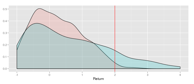
Let’s start by refreshing our memory of “reaching for yield”. In his February speech, Jeremy Stein argued that because many institutional investors need to meet nominal return requirements, these investors were reaching into riskier assets. Even though these assets may not offer high expected returns, their variance profiles offer better chances of hitting the nominal requirement. This game of distributions is illustrated below. Even though the safe red (i.e. low variance) asset has a higher expected return, the risky blue (high variance) asset has a better chance of getting the fund manager over the critical red required return line. As a result, a market wide reach for yield may result in a mispricing of risk, jeopardizing financial stability.

These arguments have been echoed by many other commentators. Here’s Martin Feldstein in the WSJ using the reach for yield as an argument to taper:

Although the economy is weak, experience shows that further bond-buying will have little effect on economic growth and employment. Meanwhile, low interest rates are generating excessive risk-taking by banks and other financial investors. These risks could have serious adverse effects on bank capital and the value of pension funds. In Fed Chairman Ben Bernanke's terms, the efficacy of quantitative easing is low and the costs and risks are substantial.

And here’s Rajan in a speech at the Bank of International Settlements

If effective, the combination of the "low for long" policy for short term policy rates coupled with quantitative easing tends to depress yields across the yield curve for fixed income securities. Fixed income investors with minimum nominal return needs then migrate to riskier instruments such as junk bonds, emerging market bonds, or commodity ETFs, with some of the capital outflow coming back into government securities via foreign central banks accumulating reserves. Other investors migrate to stocks. To some extent, this reach for yield is precisely one of the intended consequences of unconventional monetary policy. The hope is that as the price of risk is reduced, corporations faced with a lower cost of capital will have greater incentive to make real investments, thereby creating jobs and enhancing growth.

Indeed, Bernanke felt it was necessary to address these financial stability concerns at his February and May testimonies. He argued that even if low rates encourage a reach for yield, the only way to get sustainable rates in the long run is to keep rates low now. In the metaphor of Kochlerata, you need to keep the coat on until you are warm enough to take it off.

Bernanke can rest easy. Financial data since his testimonies has even further strengthened the arguments against a reach for yield. To see why, it is important to remember two stylized facts. First, "reach for yield" is a story about financial stability. Because people are going into riskier assets, this results in a systematic underpricing of risk. Second, it’s a story about increasing risk appetites. Excessively low interest rates trigger a flight *from* quality as fund managers look to hit their nominal return requirements.

But recent moves in equity prices contradict this story. The WSJ observes that defensive sectors are underperforming.

He said he still favors stocks over bonds, and has avoided "bond proxies" such as utilities, real- estate investment trusts, and other sectors with high dividend payouts. 

Those areas are "really expensive, and they have little to no earnings growth. They have benefited hugely from easing," he said. 

Those traditionally defensive sectors dragged on benchmarks. The sole decliners in late trading were the utilities and consumer-staples sectors, which lost 0.9% and 0.3%, respectively. Those areas were among the biggest gainers in the beginning of the year, when yields on Treasury bonds remained low.

Whereas cyclicals are responding very well:

Given the cross currents in the market, including the Fed's commitment to keeping overnight rates low at least until the unemployment rate falls through 6.5%, investors wouldn't want to overinterpret what's happened to the yield curve. But the stock market told a similar story of stronger growth expectations Friday. Shares of economically sensitive companies, like banks, retailers and manufacturers, rallied, while defensive areas, like utility and telecom shares, did poorly.

In other words, the recent taper has caused people to pivot out of safe sectors into riskier ones -- the opposite of what a reach for yield story would suggest. In fact, there appears to have been a flight *to* quality that is only recently being reversed. These movements are also consistent with recent data showing the equity risk premium, or a measure of stock market performance relative to the bond market, is at extremely elevated levels. With the taper we should expect this premium to fall as investors naturally increase their risk appetites.

Now, some may argue that there was a reach for yield in the fixed income market that is now being unwound. Indeed, mortgage rates and junk bond yields are rising:

Rates on a 30-year mortgage have climbed from 3.45% in April to more than 4% in June, according to Freddie Mac FMCC +1.97% . The 30-day average yield on new bonds sold by companies with "junk" credit ratings hit 7.72% in June, up from 5.79% in April, according to S&P Capital IQ LCD.

The risk premium on high yield bonds has also risen slightly. But there are two reasons why we should discount this observation.

First, the bond spreads will have a minimal effect on financial stability. The concern shouldn't be whether individual funds will suffer, but rather whether there has been a massive mispricing in risk. But if the risk was underpriced in the debt market, then the equity prices should have been overpriced to match the artificially low cost of capital. However, since there did not appear to be a reach for equity yield, then any reach for yield in fixed income should also have negligible effects.

Second, the high yield spread is still not outside of its historical range. Even in the 1990’s, when the Fed was never criticized for promoting a reach for yield, the spread was still very low. Therefore we should be skeptical of arguments that there was a massive mispricing in the corporate debt market to begin with.

This perspective from the reach for yield debate leads to two insights.

First, Fed policy has not been distorting financial markets. If anything, people have been too conservative on equities. Monetary policy, by encouraging risk taking, has been doing the right thing to do to help reboot the market. Even if you don’t want firms reaching for yield, they should at least be encouraged to stretch.

Second, it’s not clear if the taper will be all that “terrible” for equities. Of course, the human cost of tight monetary policy is enormous. I personally believe that the Fed should not taper in the face of such elevated levels of unemployment and depressed levels of nominal GDP. Nonetheless, the taper is likely to have only moderate impacts on the stock market, in spite of what short term correlations may suggest.

The greatest irony is that only after the Fed tightens do we realize that the Fed didn’t need to tighten at all. But now that it has, it doesn’t look like the financial impacts will be that large after all.

The Role of Financial Institutions

The real world of finance is not populated by the financial traders of model fame. Numerous studies in behavioral economics have identified what appear to be deviations from fully efficient markets with rational individuals. On the individual level, we know that overconfidence leads male traders to trade much more than female traders, and this has a negative effect on their returns. Therefore agents don’t seem to be optimizing -- rather they have their own idiosyncratic, but systematic, biases. On the market level, stock prices seem to exhibit strong short-run momentum while also appear to have long-run mean reverting growth rates. This suggests that there’s something going on with market participants that encourages overshooting in the short run but with corrections in the long run. 

But what has gotten me curious over the past few months is the institutional aspect. In my view, because financial markets are actually populated by institutions that have their own quirks, financial markets can deviate from textbook models in very policy relevant ways.

Most financial models that I have read about are populated by individual investors looking to maximize some expected future consumption stream subject to various constraints. Sometimes these constraints stick to describing feasible budget allocations,and sometimes they also include cognitive biases. But Wall Street doesn't look like this. Traders rarely trade by themselves -- they are usually a part of a large firm. These firms may also have different goals. Some, such as hedge funds, are just in the business of generating pure return whereas others, such as pension funds, are looking to maintain a steady stream of payments to pay out to their customers. Given that these firms have their own institutional demands, this suggests that their trading strategies could be quite different. These structural differences has implications for market efficiency.

Past papers have of course addressed some of these issues. On a within-firm basis, work on the principal-agent problem has shown how compensation schemes can affect fund manager behavior. This would suggest that many financial managers maximize not the utility of the investor, but their payoff in the compensation scheme. Some past work has also indicated that institutional investors, in this case mostly pension funds, do not seem to exhibit the herding and destabilizing behavior that for which they are criticized. However, some of these benign results are being challenged in the recent financial crisis, and this could have major implications for both financial research and monetary policy.

As an example, there have been a set of recent popular articles from the Economist and FT Alphaville on the notion of VAR shocks. VAR is a measure of financial risk that (theoretically) measures the worst case outcome for a firm. For example, a 5% weekly VaR of $5 million means that there should only be a 5% percent chance that the firm will lose more than $5 million over the course of a given week. This typically can be calculated by parameterizing a loss distribution with historical data on volatility and average yields. Even though this measure can mislead by ignoring the amount that would actually be lost in a worst-case outcome its simplicity makes it a natural candidate for institutions to use as a check against overly risky trading strategies. Therefore market moves that can impact the measurement of VAR are natural candidates for making the institutional investors jump.


Pioneering work by Hyun Song Shin, an economist at Princeton, analyzes the role of VAR and argues that it contributes to market procyclicality. Because historical data is used to calculate the VAR that goes into risk weighting, banks may end up levering up their balance sheet just as the business cycle starts to rev up and deleveraging just as the entire cycle comes crashing down. The rising tide of the business cycle makes their VAR look much smaller, therefore allowing them to put smaller risk weights on their assets. Now that the size of risk weighted assets has fallen, banks can play the risk-weighting clause on capital requirements and fund themselves through more debt. This continues until the cycle breaks, at which point VAR measurements are shocked upward by the historical data, forcing a deleveraging in order to meet capital requirements, thereby amplifying negative effects on the business cycle. In particular, this story fits the recent financial crisis very well. Past decades of relative calm made the VAR models docile and ready for the slaughter that was 2008.

I see this as an institutional bug because there’s no efficiency reason why VAR should be used in such a way to risk-weight assets. It does not make for an omniscient Q-measure to identify risk. Rather, VAR is useful because it helps institutions streamline their risk analysis. By doing so, it quite possibly improves an individual firm’s performance by avoiding worse evaluation methods. But with the procyclicality argument made above, it should be clear that a group of banks all using VAR to risk weight their assets end up creating severe negative externalities on the business cycle.

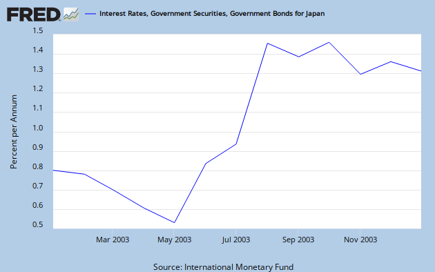
VAR shocks have also popped up in the Japanese case. Back in the 2003 bond yield volatility spike, many Japanese banks ended up selling bonds as the volatility triggered their VAR limits. This intensified the cycle of bond selling until other investors, such as pension funds and insurance companies bought up the bonds and stabilized the market. This serves as another real world example of Shin’s theory that the use of VAR in institutional settings ends up intensifying market volatility.

It should also be clear that the institutional quirks can occur in financial markets with rational arbitrageurs. If the size of institutional flows are large enough, then it may be worthwhile for the smaller traders to just ride the flows to higher returns. There may just not be enough incentive to normalize prices. If the market can stay irrational longer than individuals can stay solvent, then an individual is likely better off to just play along with the market. Given thta we see this kind of serial correlation with hedge funds in the tech bubble, the risk of individuals riding along with the irrationalities of institutions should be taken seriously. In fact, I would go far enough as to argue that the burden of proof is on those who would like to defend their financial models with only individual investors. Given that we know the real world doesn’t work like that, and that this difference can result in dramatically different conclusions, the burden must on the traditionalists to show that models of individual investing can subsume those of institutions in most cases.

To measure these effects and to calibrate new models, attention should be focused on the flow of funds in and out of these institutional investments. This way we could have a better notion of relative size and be able to measure if and how much institutional procyclicality affects markets.

I see two main policy implications of this alternative approach. First, the VAR specific quirks create a further justification for strict capital requirements. Only this way can the risk weighting problem be robustly solved. In terms of monetary policy, a thorough understanding of these institutional quirks can help guide the direction of policy. As monetarism starts to integrate more markets as data points, it becomes more and more important for central bankers to know how to interpret the financial data that comes in. By knowing what’s signal and what’s noise, central banks can better conduct forward looking policy.

In all these examples, we see how institutions -- not individual traders -- can end up driving markets. This marks a departure from traditional finance models in which everybody is just an individual playing the market. It is my hope that this kind of analysis will be useful for understanding causes of market inefficiencies and the optimal framework for financial data in monetary policy.

Why Nominal GDP Targeting Solves the Credibility Problem

Monetary easing at the zero lower bound seems to work in practice. But does it work in theory?

In his recent BIS speech, Rajan argues that monetary policy at the zero lower bound requires an impossible commitment. For the Fed to get real rates low enough for the economy to "lift-off", the only option is to raise expectations of future inflation. But what happens when that future arrives? Now that the economy has escaped the zero lower bound, the Fed is tempted to renege and stick to the original inflation target. Market participants, knowing this, then refuse to believe the original commitment, leaving the Fed stuck.

The same argument was made in reverse to explain why the Fed could not escape the high inflation equilibrium of the 1970's. As argued by Barro and Gordon, the Fed declares that it wants low inflation. If this is credible, then agents lower their expectations of inflation. However, this tempts the Fed into actually delivering high inflation to exploit the Philips curve relation and lower unemployment. As a result, the Fed is stuck at high inflation.

But the Fed escaped. The last release of the PCE price index came in at just 1.0% year over year, suggests that, if anything, the Fed lowered inflation too much. How did policy do this? In the case of moving from high inflation to low inflation, the solution was simple: adopt an inflation target. If the Fed only has to keep inflation from deviating from a target, then of course it will not cheat with any kind of surprise inflation. This kind of target can also be self reinforcing through a reputation mechanism, as the Fed knows that if it cheats now it will hurt more in the future. This removes the temptation to renege as unemployment deviations no longer matter. In the end, the Fed was successful. It managed to lower inflation from around 8% in the 1970's to the 2% levels we see today.

The target is just as important today. If the entire goal is to keep inflation at 2%, then of course there can be no commitment to forward guidance! But that is a criticism of inflation targeting, not forward guidance. Therefore the Fed needs to change its policy target. If the Fed decides its operating procedure no longer is to keep inflation at 2%, but rather to keep nominal GDP on a 5% trend, this drastically changes the perception of what is credible. The Fed no longer needs to "credibly promise to be irresponsible" -- it can just change the definition of responsibility.

If it seems magical that the Fed can change this definition so easily, it's because the loss functions that underpin these models of time inconsistency are arbitrary. In the Barro and Gordon case, the reason low inflation was time inconsistent was because unemployment deviations were included. Once the Fed ignored unemployment, its actions were time consistent. In the current forward guidance case, the reason high inflation is inconsistent is because the inflation rate is in the loss function. Therefore replacing inflation with a nominal GDP term would solve the time inconsistency problem now. The Fed gets to determine these costs. With the right loss function, credible policy becomes almost obvious.

The government can take steps towards this in many different ways. On the Fed side, they could come out with announcements saying that they are more concerned about stabilizing certain level variables -- for example nominal GDP. This would show that the Fed's loss function is changing, and therefore the expected policy adjusts. On the congressional side, they could pass a law that defines the dual mandate in terms of a nominal GDP target. This institutional reform would make Fed commitments to low future rates credible and help pull them out of the zero lower bound.

When nominal GDP targeting is cast as a framework for making future paths of interest rates credible, the implementation details of a nominal GDP target also become self evident. It's no longer a "whatever it takes" target, rather it becomes a template for adjusting the nominal interest rate. Raise the policy rate if nominal GDP is above trend, lower the rate if it's below. And if nominal GDP is so far below trend that your interest rate is stuck at zero, then provide forward guidance that the interest rate will be at zero until nominal GDP normalizes. Even though this is about future policy, there is no commitment problem. The promise is already optimal.

Therefore, nominal GDP target can make policy on the monetary instrument even more rule based. A well-defined target may make unconventional policies such as quantitative easing unnecessary -- forward guidance would be able to deliver similar results. As evidence, the recent whispers of Fed tapering have shown up most strongly in the forecasts of future interest rates. While this might seem peculiar because the Fed has not said anything about future rates, it is natural if QE is seen as a signal of the Fed's stance on future rates. Gavyn Davies notes:

There is evidence that this signalling effect of Fed balance sheet changes might be very powerful. If the Fed is not willing to “put its money where its mouth is” by buying bonds, then the market might take its promises to hold short rates at zero less seriously than before. According to this recent research by the San Francisco Fed, it is possible that a sizeable proportion of the total effect of QE on bond yields came from these signalling effects rather than the portfolio balance effects which have usually been emphasised by the central banks.

If this is the case, then the credibility effect of a nominal GDP target on forward guidance would be enough. Long rates across the board -- MBS, treasury, corporate debt -- could be lowered merely by the expected future path of rates without direct Fed intervention into those markets. Note that because inflation targeting would suffer from credibility issues when it comes to forward guidance, it can get stuck with a persistently negative output gap. This may end up forcing policy makers to deviate from the rule. So surprisingly, nominal GDP targeting would actually be more rule-based as a result.

Credibility is no problem at the zero lower bound. A nominal GDP target would go a long ways towards securing it -- in both practice and theory.