Micro and Macro Benefits Should Stay Separate

Recent posts by Mark Thoma and Michael Roberts have spurred me to think more about how to evaluate fiscal policies at the zero lower bound. Both Thoma and Roberts make arguments that because crowding out is less severe at the zero lower bound, certain government investments become much more desirable. For Thoma, this policy is increased infrastructure investment, whereas Roberts focuses more on investments in environmental policy. As such, Roberts asks: “how do we more generally evaluate the costs and benefits of public policies in a depressed economy?” This post will be an attempt at answering that question. My core thesis is that while government investment can be more desirable at the zero lower bound, it is no more desirable when the economy is at the zero lower bound than when it is not.

Why is the zero lower bound important anyways? One argument against fiscal policy is that government spending can crowd out private spending, leaving net expenditure unchanged. This can happen through two ways. First, it can happen through direct channels -- when the government builds a new school, this may crowd out a private school that was built in the region. Second, there is an interest rate channel. To finance the new spending, the government has to borrow from financial markets, crowding out private borrowing and thereby attenuating any positive effect of fiscal policy. However, when the economy is at the zero lower bound, private investment is typically weak and interest rates are low. These conditions mean that government spending will likely result in “crowding in” as multiplier effects stimulate more activity. This was the major argument behind the  DeLong and Sumner paper about fiscal policy at the zero lower bound. Therefore government investment spending carries a “double dividend” at the zero lower bound; it boosts output, long run growth, while also avoiding crowding out effects.

I see two major problems with this argument. First, it ignores the Sumner Critique about monetary policy offset. If monetary policy controls the nominal growth path of an economy, then there’s no point in trying to get more aggregate demand with government investments. Any multiplier effect will just be canceled out by the monetary authority passively tightening in response. While we haven’t seen as much tightening in the U.S. economy, we have seen this process work in reverse. Even as the government has severely tightened fiscal policy, signs of aggregate demand have held surprisingly steady. A comparison with Europe -- a continent going through a similarly savage bout of austerity -- leads us to conclude that monetary policy still has a wide latitude in determining aggregate demand even at the zero lower bound. Japan’s recent spike in growth has also shown that monetary policy can have an effect even after a long period of zero rates. This contradicts the assumption made in the DeLong and Summer paper that assumes monetary policy becomes powerless at the zero lower bound, means that any multiplier effects of government investment are minimal. Therefore multiplier or “crowding in” effects do not serve as a sound basis for evaluating government investment.

Now suppose for some reason that the monetary authority has imperfect credibility and cannot pull the economy out of the zero lower bound. Does government investment become more attractive as a result? Still no. This is because the proper benchmark is not the absence of government spending, but rather the next best government spending option. When considering all these investment proposals, we should remember that the government could always spend its money on “firework shows” or “alien defenses”. This (inefficient) policy scheme would capture all the multiplier expenditure effects with none of the long run growth effects. But as a result, the dividend of using government investment are no greater at the zero lower bound than when interest rates are positive.

Some others have made the even more radical argument that the zero lower bound means aggregate supply reducing policies, such as more stringent environmental regulations, can actually have macro benefits at the zero lower bound by increasing inflation. However, a look at forecast data in Japan around the time of the tsunami and in the U.S. around the time of the Libyan oil shocks shows that adverse supply shocks are, well, adverse. Output doesn't rise in response to supply shocks -- even at the zero lower bound.

So where do we end up? While the “double dividend” hypothesis might be a strong political argument for government investment, the core, apolitical economic analysis suggests that the zero lower bound does not make investment more desirable than usual. As a result, focus needs to be directed towards identifying the efficiency costs of low investment, not low output -- focus on the Harberger triangles, not the Okun gaps.

The Taper and Growth -- A Reply to Brad DeLong

Intellectual honesty means disagreeing with even those who are “on my side”. So when the arguments I have made against Reaching for Yield are also arguments against doomsday predictions for the taper, I have to speak up.

In this case, I have Brad DeLong in mind. In a post today, Brad sees the recent rise in real interest rates as measured by the 10 Year TIPS yield and the fall in inflation expectations as measured by the 10 year breakeven as cause for alarm, claiming that “Not since 1991 have we had such a large and rapid contractionary shift in the market's belief about what the Federal Reserve's reaction function.”

Reading his post, it almost sounds like Fed policy is going to collapse growth. But I would argue that while Fed policy is failing to promote maximum employment, it hardly follows that growth will collapse. I come to this conclusion also by looking at financial data. Below I reproduce a plot of the real interest rate, inflation breakeven (both 10 year), and add a plot of the SP500. I focus in on 2013 to see the recent dramatic changes.



We can make some stylized observations. First, the real interest rate has been on a steady rise since May. Second, the inflation breakeven has been on secular decline since about March. Third, in spite of all of this, the SP500 has been steadily growing, rising more than 10% on a year to date basis.

How should we interpret this? If we accept the uncontroversial proposition that stock market movements reflect expectations of future growth, it should be clear that the fall in inflation expectations does not reflect a fall in expected future nominal GDP. This is a break from the trends from 2010 to 2012. But if inflation is not moving in the same direction in output, it must be that a positive supply shock is the driving factor behind the fall in inflation breakevens.

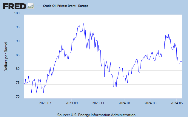
The natural candidate for the positive supply shock is the fall in oil prices. The recent slowdown in emerging markets and massive expansion in oil production has lowered energy costs for the United States. This is a textbook expansion in aggregate supply, and we should naturally expect output to rise, inflation to fall -- precisely what we observe above.



Nonetheless, I still agree that more monetary stimulus is desired. To see this, we should consider the first differences in inflation expectations and the SP500. In the plot below, I have plotted weekly percent changes in the inflation breakeven and the SP500. Blue denotes points in the 2010-2012 time period, and red denotes the points on a year to date basis. Note that in both samples there is a positive relationship between changes in inflation expectations and changes in the SP500. However, the year to date group has a higher intercept, reflecting that the SP500 has shifted to a higher trend growth path relative to the 2010-2012 period. Indeed, if you run the regressions on the first differences, you find that in the 2010-2012 period, the SP500 would gain only 0.23% in a week if inflation expectations were unchanged. However, in 2013, the value is 0.76% -- almost triple what the previous trend growth rate.

These facts show the simplest version of the aggregate supply/aggregate demand model in action. If inflation falls while nominal GDP rises, then it must be a positive supply shock. For every level of inflation we achieve a higher level of output. But even after the positive supply shock, aggregate demand policy still plays a role -- i.e. any marginal rise in inflation still translates to a rise in output.

What went wrong in DeLong’s original analysis was that he reasoned from a price change. He started by talking about inflation and interest rates and then translated that into a statement about monetary policy. On the other hand, I started with a quantity -- the SP500 -- and used that to interpret the price changes. This allows me to fit the data into the standard AS/AD model.

I can then break down potential data changes to events in the AS/AD model. DeLong writes out a list of four possibilities to interpret changes in the real interest rate and the inflation breakeven. II have produced a similar table below that translate the AS/AD arguments I made above. My version provides endogenous predictions for the real interest rate -- the market indicators are inflation expectations and the SP500.

In my view, the economy is in state (4). Inflation is weak, but growth will be strong. These growth prospects are also corroborated by the relative strength of cyclical stock sectors relative to safe ones. Investors are ramping up -- not buckling down -- as expectations of future nominal GDP rise. Bottom line? The taper isn't going to knock growth far off track.

This rate story shows how important markets are in market monetarism, TIPS spreads and movements in the SP500 make for an easy breakdown of aggregate supply aggregate demand. We should take them seriously, even if it’s politically inconvenient for those of us arguing for monetary easing. Interest rate movements signal changes in the reactions of the Fed. But since it's unlikely that the Fed will screw up so badly so as to have elevated interest rates for an extended period when the economy is suffering, rising long rates almost always indicate higher expected nominal GDP. These financial indicators provide policy makers with forward looking data on which to base policy -- a cornerstone of market monetarism.

I want to end on what the above means for monetary policy and advocates of monetary easing, such as myself.

First, the recent fall in inflation breakevens should not be interpreted as a monetary tightening -- the change is not being driven by demand, but rather by supply. Second, the Fed is severely failing its dual mandate. Now that inflation is falling, the Fed should have even more latitude to pursue its full employment objectives. In this light, the taper is madness. Third, advocacy for monetary easing should focus on the human costs, not financial costs, of tight money. Wall Street will move on, but Fed complacency in the face of half a decade of slow job growth will leave scars on Main Street for years to come.

Debt Is Not Damning. Debt is Just Debt

This post is meant to add a little few final goodies to the work I did with Miles Kimball on the Reinhart and Rogoff results. In short, Miles and I took another look at the RR dataset as prepared by Herndon et al. and found that the long run effects of debt on growth were vanishingly small. The major innovation driving our finding was to look not at contemporaneous growth, but rather at growth 5 to 10 years out in either direction. We ended up finding that while low past growth does a good job of predicting high current debt, current debt does a rather poor job predicting low future growth.

The column had a very strong response, and as such we each had a few follow up posts. Immediately after the first article, Miles started addressing new points brought up by various commentators, and these can be seen here. I later wrote about controlling for the possibility that policy makers would manipulated their debt levels in expectation of future growth rates, and Miles had a post on the importance of taking enough lags of growth rates into account. We pursued these ideas further in another Quartz article that featured (in my opinion) a very good looking scatterplot that lets you see the individual countries that contribute to the regression results.

Since part of this controversy was over data sharing practices, I made sure to make all the code available in the Data section of my blog.

Before presenting the original article, I want to add two more pictures to the debate. The first is a scatter plot that breaks down the relationships between future growth, past growth, and debt by both country and time -- something that Evan Soltas asked for when the article was released. These diagrams show that even when the observations are grouped by decade, the general conclusion that debt does not slow future growth  still holds. This plot also allows you to see which countries are the influential outliers. With any luck, this granularity can inspire some more posts about what the experiences of those individual countries can teach us about debt and growth.

To me, what is most stark about these plots is that the Solow growth model implies both panels should have downward sloping lines. Since debt levels usually rise as countries approach the technological frontier and start welfare states, we should expect debt to be negatively correlated with growth -- both past and future. Therefore the nearly flat slopes in the left panel really do suggest debt's effect on future growth is quite small.

As a second plot on this point, I want to present a version of the debt/gdp buckets plot because that nonparametric approach  was a big part of the RR debt/growth message. It turns out that as soon as we look at future growth, the buckets no longer show much of a slowdown at all at moderate levels of growth. However, the buckets maintain the robust negative relationship between past growth and current debt. Even though this image might be provocative, I would  recommend not reading too much into it. The standard errors should be quite large and are not included, and none of these bar charts adjust for past growth.

And now, the full text of the article. If you want to mirror the content of this post on another site, that is possible for a limited time if you read the legal notice at this link and include both a link to the original Quartz column and the following copyright notice:

© May 29, 2013: Miles Kimball and Yichuan Wang, as first published on Quartz. Used by permission according to a temporary nonexclusive license expiring June 30, 2014. All rights reserved.

---

After Crunching Reinhart and Rogoff’s Data, We Found No Evidence High Debt Slows Growth

Miles Kimball and Yichuan Wang

Leaving aside monetary policy, the textbook Keynesian remedy for recession is to increase government spending or cut taxes. The obvious problem with that is that higher government spending and lower taxes tend to put the government deeper in debt. So the announcement on April 15, 2013 by University of Massachusetts at Amherst economists Thomas Herndon, Michael Ash and Robert Pollin that Carmen Reinhart and Ken Rogoff had made a mistake in their analysis claiming that debt leads to lower economic growth has been big news. Remarkably for a story so wonkish, the tale of Reinhart and Rogoff’s errors even made it onto the Colbert Report. Six weeks later, discussions of Herndon, Ash and Pollin’s challenge to Reinhart and Rogoff continue in earnest in the economics blogosphere, in the Wall Street Journal, and in the New York Times.

In defending the main conclusions of their work, while conceding some errors, Reinhart and Rogoff point out that even after the errors are corrected, there is a substantial negative correlation between debt levels and economic growth. That is a fair description of what Herndon, Ash and Pollin find, as discussed in an earlier Quartz column, “An Economist’s Mea Culpa: I relied on Reinhardt and Rogoff.” But, as mentioned there, and as Reinhart and Rogoff point out in their response to Herndon, Ash and Pollin, there is a key remaining issue of what causes what. It is well known among economists that low growth leads to extra debt because tax revenues go down and spending goes up in a recession. But does debt also cause low growth in a vicious cycle? That is the question.

We wanted to see for ourselves what Reinhart and Rogoff’s data could say about whether high national debt seems to cause low growth. In particular, we wanted to separate the effect of low growth in causing higher debt from any effect of higher debt in causing low growth. There is no way to do this perfectly. But we wanted to make the attempt. We had one key difference in our approach from many of the other analyses of Reinhart and Rogoff’s data: we decided to focus only on long-run effects. This is a way to avoid getting confused by the effects of business cycles such as the Great Recession that we are still recovering from. But one limitation of focusing on long-run effects is that it might leave out one of the more obvious problems with debt: the bond markets might at any time refuse to continue lending except at punitively high interest rates, causing debt crises like that have been faced by Greece, Ireland, and Cyprus, and to a lesser degree Spain and Italy. So far, debt crises like this have been rare for countries that have borrowed in their own currency, but are a serious danger for countries that borrow in a foreign currency or share a currency with many other countries in the euro zone.

Here is what we did to focus on long-run effects: to avoid being confused by business-cycle effects, we looked at the relationship between national debt and growth in the period of time from five to 10 years later. In their paper “Debt Overhangs, Past and Present,” Carmen Reinhart and Ken Rogoff, along with Vincent Reinhart, emphasize that most episodes of high national debt last a long time. That means that if high debt really causes low growth in a slow, corrosive way, we should be able to see high debt now associated with low growth far into the future for the simple reason that high debt now tends to be associated with high debt for quite some time into the future.

Here is the bottom line. Based on economic theory, it would be surprising indeed if high levels of national debt didn’t have at least some slow, corrosive negative effect on economic growth. And we still worry about the effects of debt. But the two of us could not find even a shred of evidence in the Reinhart and Rogoff data for a negative effect of government debt on growth.

The graphs at the top show show our first take at analyzing the Reinhardt and Rogoff data. This first take seemed to indicate a large effect of low economic growth in the past in raising debt combined with a smaller, but still very important effect of high debt in lowering later economic growth. On the right panel of the graph above, you can see the strong downward slope that indicates a strong correlation between low growth rates in the period from ten years ago to five years ago with more debt, suggesting that low growth in the past causes high debt. On the left panel of the graph above, you can see the mild downward slope that indicates a weaker correlation between debt and lower growth in the period from five years later to ten years later, suggesting that debt might have some negative effect on growth in the long run. In order to avoid overstating the amount of data available, these graphs have only one dot for each five-year period in the data set. If our further analysis had confirmed these results, we were prepared to argue that the evidence suggested a serious worry about the effects of debt on growth. But the story the graphs above seem to tell dissolves on closer examination.

Given the strong effect past low growth seemed to have on debt, we felt that we needed to take into account the effect of past economic growth rates on debt more carefully when trying to tease out the effects in the other direction, of debt on later growth. Economists often use a technique called multiple regression analysis (or “ordinary least squares”) to take into account the effect of one thing when looking at the effect of something else. Here we are doing something that is quite close both in spirit and the numbers it generates for our analysis, but allows us to use graphs to show what is going on a little better.

The effects of low economic growth in the past may not all come from business cycle effects. It is possible that there are political effects as well, in which a slowly growing pie to be divided makes it harder for different political factions to agree, resulting in deficits. Low growth in the past may also be a sign that a government is incompetent or dysfunctional in some other way that also causes high debt. So the way we took into account the effects of economic growth in the past on debt—and the effects on debt of the level of government competence that past growth may signify—was to look at what level of debt could be predicted by knowing the rates of economic growth from the past year, and in the three-year periods from 10 to 7 years ago, 7 to 4 years ago and 4 to 1 years ago. The graph below, labeled “Prediction of Debt Based on Past Growth” shows that knowing these various economic growth rates over the past 10 years helps a lot in predicting how high the ratio of national debt to GDP will be on a year by year basis. (Doing things on a year by year basis gives the best prediction, but means the graph has five times as many dots as the other scatter plots.) The “Prediction of Debt Based on Past Growth” graph shows that some countries, at some times, have debt above what one would expect based on past growth and some countries have debt below what one would expect based on past growth. If higher debt causes lower growth, then national debt beyond what could be predicted by past economic growth should be bad for future growth.

Our next graph below, labeled “Relationship Between Future Growth and Excess Debt to GDP” shows the relationship between a debt to GDP ratio beyond what would be predicted by past growth and economic growth 5 to 10 years later. Here there is no downward slope at all. In fact there is a small upward slope. This was surprising enough that we asked others we knew to see what they found when trying our basic approach. They bear no responsibility for our interpretation of the analysis here, but Owen Zidar, an economics graduate student at the University of California, Berkeley, and Daniel Weagley, graduate student in finance at the University of Michigan were generous enough to analyze the data from our angle to help alert us if they found we were dramatically off course and to suggest various ways to handle details. (In addition, Yu She, a student in the master’s of applied economics program at the University of Michigan proofread our computer code.) We have no doubt that someone could use a slightly different data set or tweak the analysis enough to make the small upward slope into a small downward slope. But the fact that we got a small upward slope so easily (on our first try with this approach of controlling for past growth more carefully) means that there is no robust evidence in the Reinhart and Rogoff data set for a negative long-run effect of debt on future growth once the effects of past growth on debt are taken into account. (We still get an upward slope when we do things on a year-by-year basis instead of looking at non-overlapping five-year growth periods.)

Daniel Weagley raised a very interesting issue that the very slight upward slope shown for the “Relationship Between Future Growth and Excess Debt to GDP” is composed of two different kinds of evidence. Times when countries in the data set, on average, have higher debt than would be predicted tend to be associated with higher growth in the period from five to 10 years later. But at any time, countries that have debt that is unexpectedly high not only compared to their own past growth, but also compared to the unexpected debt of other countries at that time, do indeed tend to have lower growth five to 10 years later. It is only speculating, but this is what one might expect if the main mechanism for long-run effects of debt on growth is more of the short-run effect we mentioned above: the danger that the “bond market vigilantes” will start demanding high interest rates. It is hard for the bond market vigilantes to take their money out of all government bonds everywhere in the world, so having debt that looks high compared to other countries at any given time might be what matters most.

Our view is that evidence from trends in the average level of debt around the world over time are just as instructive as evidence from the cross-national evidence from debt in one country being higher than in other countries at a given time. Our last graph (just above) shows what the evidence from trends in average levels over time looks like. High debt levels in the late 1940s and the 1950s were followed five to 10 years later with relatively high growth. Low debt levels in the 1960s and 1970s were followed five to 10 years later by relatively low growth. High debt levels in the 1980s and 1990s were followed five to 10 years later by relatively high growth. If anyone can come up with a good argument for why this evidence from trends in the average levels over time should be dismissed, then only the cross-national evidence about debt in one country compared to another would remain, which by itself makes debt look bad for growth. But we argue that there is not enough justification to say that special occurrences each year make the evidence from trends in the average levels over time worthless. (Technically, we don’t think it is appropriate to use “year fixed effects” to soak up and throw away evidence from those trends over time in the average level of debt around the world.)

We don’t want anyone to take away the message that high levels of national debt are a matter of no concern. As discussed in “Why Austerity Budgets Won’t Save Your Economy,” the big problem with debt is that the only ways to avoid paying it back or paying interest on it forever are national bankruptcy or hyper-inflation. And unless the borrowed money is spent in ways that foster economic growth in a big way, paying it back or paying interest on it forever will mean future pain in the form of higher taxes or lower spending.

There is very little evidence that spending borrowed money on conventional Keynesian stimulus—spent in the ways dictated by what has become normal politics in the US, Europe and Japan—(or the kinds of tax cuts typically proposed) can stimulate the economy enough to avoid having to raise taxes or cut spending in the future to pay the debt back. There are three main ways to use debt to increase growth enough to avoid having to raise taxes or cut spending later:

1. Spending on national investments that have a very high return, such as in scientific research, fixing roads or bridges that have been sorely neglected. 

2. Using government support to catalyze private borrowing by firms and households, such as government support for student loans, and temporary investment tax credits or Federal Lines of Credit to households used as a stimulus measure. 

3. Issuing debt to create a sovereign wealth fund—that is, putting the money into the corporate stock and bond markets instead of spending it, as discussed in “Why the US needs its own sovereign wealth fund.” For anyone who thinks government debt is important as a form of collateral for private firms (see “How a US Sovereign Wealth Fund Can Alleviate a Scarcity of Safe Assets”), this is the way to get those benefits of debt, while earning more interest and dividends for tax payers than the extra debt costs. And a sovereign wealth fund (like breaking through the zero lower bound with electronic money) makes the tilt of governments toward short-term financing caused by current quantitative easing policies unnecessary.

But even if debt is used in ways that do require higher taxes or lower spending in the future, it may sometimes be worth it. If a country has its own currency, and borrows using appropriate long-term debt (so it only has to refinance a small fraction of the debt each year) the danger from bond market vigilantes can be kept to a minimum. And other than the danger from bond market vigilantes, we find no persuasive evidence from Reinhart and Rogoff’s data set to worry about anything but the higher future taxes or lower future spending needed to pay for that long-term debt. We look forward to further evidence and further thinking on the effects of debt. But our bottom line from this analysis, and the thinking we have been able to articulate above, is this: Done carefully, debt is not damning. Debt is just debt.

Where did the Reach for Yield Go?

Friday’s strong data caused bond yields to spike. This has caused some consternation from economic commentators, and Paul Krugman in particular has argued that the rise in interest rates will have severe economic impacts. While I want to touch on these issues, I will approach them from a different debate -- that over the "reach for yield". My thesis? The recent rebalancing in the stock market shows that the reach for yield was overstated, and that, from this, we can conclude the taper will not have a severe negative effect on growth.

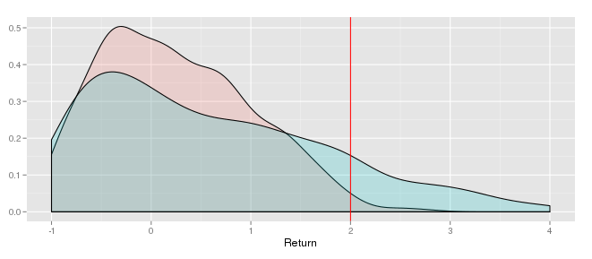
Let’s start by refreshing our memory of “reaching for yield”. In his February speech, Jeremy Stein argued that because many institutional investors need to meet nominal return requirements, these investors were reaching into riskier assets. Even though these assets may not offer high expected returns, their variance profiles offer better chances of hitting the nominal requirement. This game of distributions is illustrated below. Even though the safe red (i.e. low variance) asset has a higher expected return, the risky blue (high variance) asset has a better chance of getting the fund manager over the critical red required return line. As a result, a market wide reach for yield may result in a mispricing of risk, jeopardizing financial stability.

These arguments have been echoed by many other commentators. Here’s Martin Feldstein in the WSJ using the reach for yield as an argument to taper:

Although the economy is weak, experience shows that further bond-buying will have little effect on economic growth and employment. Meanwhile, low interest rates are generating excessive risk-taking by banks and other financial investors. These risks could have serious adverse effects on bank capital and the value of pension funds. In Fed Chairman Ben Bernanke's terms, the efficacy of quantitative easing is low and the costs and risks are substantial.

And here’s Rajan in a speech at the Bank of International Settlements

If effective, the combination of the "low for long" policy for short term policy rates coupled with quantitative easing tends to depress yields across the yield curve for fixed income securities. Fixed income investors with minimum nominal return needs then migrate to riskier instruments such as junk bonds, emerging market bonds, or commodity ETFs, with some of the capital outflow coming back into government securities via foreign central banks accumulating reserves. Other investors migrate to stocks. To some extent, this reach for yield is precisely one of the intended consequences of unconventional monetary policy. The hope is that as the price of risk is reduced, corporations faced with a lower cost of capital will have greater incentive to make real investments, thereby creating jobs and enhancing growth.

Indeed, Bernanke felt it was necessary to address these financial stability concerns at his February and May testimonies. He argued that even if low rates encourage a reach for yield, the only way to get sustainable rates in the long run is to keep rates low now. In the metaphor of Kochlerata, you need to keep the coat on until you are warm enough to take it off.

Bernanke can rest easy. Financial data since his testimonies has even further strengthened the arguments against a reach for yield. To see why, it is important to remember two stylized facts. First, "reach for yield" is a story about financial stability. Because people are going into riskier assets, this results in a systematic underpricing of risk. Second, it’s a story about increasing risk appetites. Excessively low interest rates trigger a flight *from* quality as fund managers look to hit their nominal return requirements.

But recent moves in equity prices contradict this story. The WSJ observes that defensive sectors are underperforming.

He said he still favors stocks over bonds, and has avoided "bond proxies" such as utilities, real- estate investment trusts, and other sectors with high dividend payouts. 

Those areas are "really expensive, and they have little to no earnings growth. They have benefited hugely from easing," he said. 

Those traditionally defensive sectors dragged on benchmarks. The sole decliners in late trading were the utilities and consumer-staples sectors, which lost 0.9% and 0.3%, respectively. Those areas were among the biggest gainers in the beginning of the year, when yields on Treasury bonds remained low.

Whereas cyclicals are responding very well:

Given the cross currents in the market, including the Fed's commitment to keeping overnight rates low at least until the unemployment rate falls through 6.5%, investors wouldn't want to overinterpret what's happened to the yield curve. But the stock market told a similar story of stronger growth expectations Friday. Shares of economically sensitive companies, like banks, retailers and manufacturers, rallied, while defensive areas, like utility and telecom shares, did poorly.

In other words, the recent taper has caused people to pivot out of safe sectors into riskier ones -- the opposite of what a reach for yield story would suggest. In fact, there appears to have been a flight *to* quality that is only recently being reversed. These movements are also consistent with recent data showing the equity risk premium, or a measure of stock market performance relative to the bond market, is at extremely elevated levels. With the taper we should expect this premium to fall as investors naturally increase their risk appetites.

Now, some may argue that there was a reach for yield in the fixed income market that is now being unwound. Indeed, mortgage rates and junk bond yields are rising:

Rates on a 30-year mortgage have climbed from 3.45% in April to more than 4% in June, according to Freddie Mac FMCC +1.97% . The 30-day average yield on new bonds sold by companies with "junk" credit ratings hit 7.72% in June, up from 5.79% in April, according to S&P Capital IQ LCD.

The risk premium on high yield bonds has also risen slightly. But there are two reasons why we should discount this observation.

First, the bond spreads will have a minimal effect on financial stability. The concern shouldn't be whether individual funds will suffer, but rather whether there has been a massive mispricing in risk. But if the risk was underpriced in the debt market, then the equity prices should have been overpriced to match the artificially low cost of capital. However, since there did not appear to be a reach for equity yield, then any reach for yield in fixed income should also have negligible effects.

Second, the high yield spread is still not outside of its historical range. Even in the 1990’s, when the Fed was never criticized for promoting a reach for yield, the spread was still very low. Therefore we should be skeptical of arguments that there was a massive mispricing in the corporate debt market to begin with.

This perspective from the reach for yield debate leads to two insights.

First, Fed policy has not been distorting financial markets. If anything, people have been too conservative on equities. Monetary policy, by encouraging risk taking, has been doing the right thing to do to help reboot the market. Even if you don’t want firms reaching for yield, they should at least be encouraged to stretch.

Second, it’s not clear if the taper will be all that “terrible” for equities. Of course, the human cost of tight monetary policy is enormous. I personally believe that the Fed should not taper in the face of such elevated levels of unemployment and depressed levels of nominal GDP. Nonetheless, the taper is likely to have only moderate impacts on the stock market, in spite of what short term correlations may suggest.

The greatest irony is that only after the Fed tightens do we realize that the Fed didn’t need to tighten at all. But now that it has, it doesn’t look like the financial impacts will be that large after all.

The Role of Financial Institutions

The real world of finance is not populated by the financial traders of model fame. Numerous studies in behavioral economics have identified what appear to be deviations from fully efficient markets with rational individuals. On the individual level, we know that overconfidence leads male traders to trade much more than female traders, and this has a negative effect on their returns. Therefore agents don’t seem to be optimizing -- rather they have their own idiosyncratic, but systematic, biases. On the market level, stock prices seem to exhibit strong short-run momentum while also appear to have long-run mean reverting growth rates. This suggests that there’s something going on with market participants that encourages overshooting in the short run but with corrections in the long run. 

But what has gotten me curious over the past few months is the institutional aspect. In my view, because financial markets are actually populated by institutions that have their own quirks, financial markets can deviate from textbook models in very policy relevant ways.

Most financial models that I have read about are populated by individual investors looking to maximize some expected future consumption stream subject to various constraints. Sometimes these constraints stick to describing feasible budget allocations,and sometimes they also include cognitive biases. But Wall Street doesn't look like this. Traders rarely trade by themselves -- they are usually a part of a large firm. These firms may also have different goals. Some, such as hedge funds, are just in the business of generating pure return whereas others, such as pension funds, are looking to maintain a steady stream of payments to pay out to their customers. Given that these firms have their own institutional demands, this suggests that their trading strategies could be quite different. These structural differences has implications for market efficiency.

Past papers have of course addressed some of these issues. On a within-firm basis, work on the principal-agent problem has shown how compensation schemes can affect fund manager behavior. This would suggest that many financial managers maximize not the utility of the investor, but their payoff in the compensation scheme. Some past work has also indicated that institutional investors, in this case mostly pension funds, do not seem to exhibit the herding and destabilizing behavior that for which they are criticized. However, some of these benign results are being challenged in the recent financial crisis, and this could have major implications for both financial research and monetary policy.

As an example, there have been a set of recent popular articles from the Economist and FT Alphaville on the notion of VAR shocks. VAR is a measure of financial risk that (theoretically) measures the worst case outcome for a firm. For example, a 5% weekly VaR of $5 million means that there should only be a 5% percent chance that the firm will lose more than $5 million over the course of a given week. This typically can be calculated by parameterizing a loss distribution with historical data on volatility and average yields. Even though this measure can mislead by ignoring the amount that would actually be lost in a worst-case outcome its simplicity makes it a natural candidate for institutions to use as a check against overly risky trading strategies. Therefore market moves that can impact the measurement of VAR are natural candidates for making the institutional investors jump.


Pioneering work by Hyun Song Shin, an economist at Princeton, analyzes the role of VAR and argues that it contributes to market procyclicality. Because historical data is used to calculate the VAR that goes into risk weighting, banks may end up levering up their balance sheet just as the business cycle starts to rev up and deleveraging just as the entire cycle comes crashing down. The rising tide of the business cycle makes their VAR look much smaller, therefore allowing them to put smaller risk weights on their assets. Now that the size of risk weighted assets has fallen, banks can play the risk-weighting clause on capital requirements and fund themselves through more debt. This continues until the cycle breaks, at which point VAR measurements are shocked upward by the historical data, forcing a deleveraging in order to meet capital requirements, thereby amplifying negative effects on the business cycle. In particular, this story fits the recent financial crisis very well. Past decades of relative calm made the VAR models docile and ready for the slaughter that was 2008.

I see this as an institutional bug because there’s no efficiency reason why VAR should be used in such a way to risk-weight assets. It does not make for an omniscient Q-measure to identify risk. Rather, VAR is useful because it helps institutions streamline their risk analysis. By doing so, it quite possibly improves an individual firm’s performance by avoiding worse evaluation methods. But with the procyclicality argument made above, it should be clear that a group of banks all using VAR to risk weight their assets end up creating severe negative externalities on the business cycle.

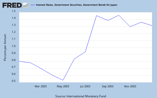
VAR shocks have also popped up in the Japanese case. Back in the 2003 bond yield volatility spike, many Japanese banks ended up selling bonds as the volatility triggered their VAR limits. This intensified the cycle of bond selling until other investors, such as pension funds and insurance companies bought up the bonds and stabilized the market. This serves as another real world example of Shin’s theory that the use of VAR in institutional settings ends up intensifying market volatility.

It should also be clear that the institutional quirks can occur in financial markets with rational arbitrageurs. If the size of institutional flows are large enough, then it may be worthwhile for the smaller traders to just ride the flows to higher returns. There may just not be enough incentive to normalize prices. If the market can stay irrational longer than individuals can stay solvent, then an individual is likely better off to just play along with the market. Given thta we see this kind of serial correlation with hedge funds in the tech bubble, the risk of individuals riding along with the irrationalities of institutions should be taken seriously. In fact, I would go far enough as to argue that the burden of proof is on those who would like to defend their financial models with only individual investors. Given that we know the real world doesn’t work like that, and that this difference can result in dramatically different conclusions, the burden must on the traditionalists to show that models of individual investing can subsume those of institutions in most cases.

To measure these effects and to calibrate new models, attention should be focused on the flow of funds in and out of these institutional investments. This way we could have a better notion of relative size and be able to measure if and how much institutional procyclicality affects markets.

I see two main policy implications of this alternative approach. First, the VAR specific quirks create a further justification for strict capital requirements. Only this way can the risk weighting problem be robustly solved. In terms of monetary policy, a thorough understanding of these institutional quirks can help guide the direction of policy. As monetarism starts to integrate more markets as data points, it becomes more and more important for central bankers to know how to interpret the financial data that comes in. By knowing what’s signal and what’s noise, central banks can better conduct forward looking policy.

In all these examples, we see how institutions -- not individual traders -- can end up driving markets. This marks a departure from traditional finance models in which everybody is just an individual playing the market. It is my hope that this kind of analysis will be useful for understanding causes of market inefficiencies and the optimal framework for financial data in monetary policy.

Capital Requirements and Nominal GDP Targeting

The Federal Reserve has recently moved to tighten capital requirements for banks, and I see this as a long overdue move. While others have done a very good job summarizing the minutiae of the various ratios, I want to explore what capital requirements really mean and, more importantly, what implications these requirements have on monetary policy.

First, we should be clear on what capital really is. Despite phrases such as “capital cushion” or “holding capital”, capital holdings are not the same as reserves. Capital is meant to describe a type of funding structure, not an asset allocation -- a liability, not an asset. So what is truly at stake here with the capital requirements debate is how banks fund themselves: through equity or debt.

The argument for higher equity funding comes down to reducing the incentive to run on the banks. Because debt liabilities are fixed, creditors are likely to demand their money back at the first sign of trouble. On the other hand, if the funding comes from equity, there is no similar compulsion to run, thereby preventing the fire sale spirals that characterise financial distress.

To visualize this, consider the following bank balance sheet. On the left we have the funding sources -- debt and equity -- and on the right we have the assets. In this first diagram, we see a bank that relies heavily on debt funding (95%) and has very little equity (5%) -- a situation characteristic of many banks today.

Figure 1: Highly Leveraged Bank

If the bank’s assets lose value and drop by a small amount, say 7%, because the debt quantities must stay constant, then all of the equity is wiped out and the bank is left insolvent. On the other hand, had the bank financed itself through mostly equity, then the bank would have stayed solvent and not all the equity would have been wiped out. There would have been less of an incentive to have a run on the debt and, in a time of financial stress, the bank would have avoided a fire sale. These examples illustrate why high levels of debt financing can be so problematic in a system of hard to calculate risks.

Figure 2: Insolvent Bank

Equity funding prevents sudden runs and insolvency. That is the key justification for stricter capital requirements. With this in mind, I now turn my attention to the relationship between these new financial regulations and monetary policy.

The most important relationship between capital requirements and monetary policy is that capital requirements make the financial stability and “reaching for yield” arguments against monetary easing so much weaker. If institutions are well capitalized, what are we scared of? Equity bubbles, like the 2000’s dot com bust, do not leave lasting damage. However, debt bubbles, such as the 2008 financial crisis, can trigger an extended period of deleveraging and general economic malaise. Much as Scott Sumner has recommended, capital requirements can help keep the finance out of macro. While I personally believe insights from the financial literature may reveal more light on the mechanisms of monetary policy, I do agree that the task of monetary policy should stay very separate from that of financial regulation. Monetary policy makers can direct the guidance of interest rates towards maintaining a stable level of nominal output, whereas financial regulators focus on making sure the banks do not fall apart. If institutions are reaching for yield, leave it for regulators to cut the arms off. The monetary authorities need not pay any attention to it.

Even if these capital requirements are not implemented, the mere prospect of them greatly weakens the case for using monetary policy for financial stability purposes by exposing a contradiction: if monetary policy is surgical enough for financial markets, why aren’t capital requirements?

In Jeremy Stein’s February speech on monetary policy and financial stability, he argued that it may be appropriate for monetary policy to prevent bubbles. One of his key justifications was that monetary policy can “[get] in all of the cracks” of financial markets to stamp out bubbles. However, this neglects the bluntness of monetary policy.

In my view, to the extent that interest rates get in all the cracks, they do so by reducing the financial edifice into rubble. But if I am wrong and if monetary policy is indeed precise enough to stamp out bubbles without collateral damage, then aren't capital requirements even more surgical? Indeed, while monetary policy can affect the entire economy’s consumption and investment behavior, the Mogdiliani-Miller theorem suggests that changes in the capital structure would barely have an effect on those macroeconomic aggregates. The greatest irony is that the financial types who support tighter monetary policy to control financial risks are often the same ones who are against stricter capital requirements. But these views are inconsistent. Capital requirements are tailored for financial regulation, and to the extent one supports the blunt use of monetary policy, one should support the strengthening of capital requirements even more.

On the other hand, while capital requirements may make the task of monetary policy easier, some have argued that the reduction in credit from the stronger capital requirements goes against the goal of expansionary monetary policy. First, I do not believe this is true on a purely finance theory basis. As has been discussed elsewhere, higher capital requirements are unlikely to increase funding costs. To the extent that they do raise funding costs, this reflects an efficient reduction in the government’s implicit subsidies for bank debt. Second, even if this were the case, we should remember that monetary policy is not credit policy. If there is a reduction in credit, the question for the monetary authorities is whether this reduces nominal GDP. Depending on that, the Fed should ease or tighten. Therefore, a well functioning monetary policy should fully offset the potential impact of credit shocks. The level of credit in an economy is a matter of financial organization, something far outside the domain of monetary policy. The Fed should adjust the path of interest rates depending on where they want to see nominal GDP go.

While the above discussions focus on how capital requirements make monetary policy easier, I also believe better monetary policy, especially through a nominal GDP target, can help make capital requirements simpler. It’s useful to remember that debt is an extremely important channel through which nominal shocks have real effects. Rarely are these bonds written with inflation indexing, so stabilizing nominal aggregates can help make satisfying capital requirements easier. Under a nominal GDP target, the size of the debt chunk of the balance sheet can stay roughly around the same level as the size of the equity chunk, reducing the amount of scrambling that can occur in financial markets as bank struggle to reach their regulatory goals.

To conclude, I should note that there is an elegance in the combination of nominal GDP targeting, a robust monetary policy regime, and high capital requirements, a robust financial regulatory regime. As Plosser recently noted:

In the context of monetary policy, I have long advocated simple, robust rules and transparent communications.2 Robust rules are important because they are intended to work well in a variety of environments. This reflects our limited knowledge about the true determinants of economic outcomes. Economists have also come to understand that using policies that are optimal in one specific economic model can often deliver very poor outcomes if that model proves incorrect. So a policy rule that operates well under a wide range of models is a better and more robust approach.

The same approach applies to the design of regulatory frameworks as well. Because the financial world is very complex, there is merit in simple, transparent regulatory solutions designed to work reasonably well in a wide range of situations. We want rules that regulators can enforce without having superhuman knowledge or foresight. However, we can predict with virtual certainty that private actors will seek to evade regulatory restrictions and taxes. This is often called "regulatory arbitrage." We also know that enforcement costs rise as firms' incentives to evade regulations increase.

In my view, simple mechanisms that are harder to evade — and even better, mechanisms that utilize market forces to discipline firm behavior — are superior to an elaborate list of rules that seeks to cover every possible outcome. Simple and transparent regulatory mechanisms make it easier for market participants to predict how regulators are likely to behave. This, in turn, makes it easier for regulators to credibly commit to implementing the regulations in a consistent manner.

Reading Plosser’s second and third paragraphs really shines light on some common issues such as commitment, credibility, and transparency that relate financial and monetary policy. For monetary policy, these qualities can help guide the expectations that give monetary policy its oomph. For financial regulation, these qualities limit the hidden fault lines that can make crises so severe. One can only hope that policy can combine these all these qualities to make a more enlightened monetary and regulatory framework.

Man of Steel: Morality as an Evolutionary Advantage

"Your sense of morality is an evolutionary disadvantage...and evolution always wins"

This post will not be about monetary policy -- it will barely be about economics. But nonetheless, after seeing Man of Steel, I thought a fun essay connecting some core concepts from game theory and our notions of morality are in order.  While none of the insights are particularly new, the specific application to Man of Steel should be, and I hope you enjoy.

The core proposition was the one uttered by the evil Kryptonian woman pictured above. Between high paced punches and knocking helicopters out of the sky, Faora-Ul uttered to Superman: “Your sense of morality is an evolutionary disadvantage...and evolution always wins.” Whether evolution always wins is an issue that I will attend to perhaps on a different occasion, but I want to address the first claim. Is a sense of morality antithetical to the survival of the fittest?

With what we know about animal behavior, the answer seems to be a resounding “no”. While it is difficult, if not impossible, to impose a natural system of morality for animals, I think a natural interpretation could be the presence of behaviors that may not be beneficial to oneself. While morality surely goes beyond self-flagellation, it does serve as a useful residual for explaining altruistic actions.

One of the most commonly evoked examples of such behavior in the animal kingdom comes from ground squirrels. These squirrels make sure to loudly alarm their kin mates of the presence of dangerous predators. On the squirrel level, this is very costly behavior because it increases the risk that a predator finds and eats the squirrel. Yet if all squirrels do this, everybody is better off. This is a classic example of the difficulty of providing public goods, as every squirrel has the incentive to free-ride off of the alarm calls of others. But if nobody makes the alarm call, then they are all at a higher risk of being eaten by an eagle. Somehow, the squirrels manage to overcome this public goods problem. There’s no Coase theorem contract, no government enforcement, yet squirrels provide the public alarm nonetheless.

Why? In this case it’s simple: kin selection. Because these ground squirrels usually spend most of their lives around family, it’s in their incentive to protect their peers in order to pass on the most amount of genes to the next generation. Under the framing of Richard Dawkin, the selflessness of the individual squirrels comes from the selfishness of a gene that may encourage the alarm calls. To see this logic, suppose there exists a squirrel with a gene that induces the alarm calls. Then his offspring are also likely to have the same gene. Because the alarm behavior serves to preserve his offspring, then this alarm gene will propagate its way through the population. Therefore, this gene selfishly works to propagate itself, even at the cost of its host squirrel. Such is the power of family.

The above explanation has an interesting analogue from public economics, in particular the analysis of firm mergers in the presence of positive externalities. For example, consider the case of two stores that need to decide on their advertising budgets. Because of their proximity, the stores are complementary in the sense that more traffic in one store means more traffic in the other. Therefore in equilibrium, if there is no cooperation, these firms will choose an inefficiently low level of advertisements because they fail to take into account the positive benefits their own ads have on the other firm. But if they merge, the merged firm can capture this positive externality. While this may seem contrived, you can think of family structure as a merger between individual squirrels. By the same logic, this genetic merger allows the family to capture the positive externality from the alarm.

One of the greatest appeals of this kin selection theory is that it yields many good out of sample predictions. The original evidence was just the basic anomaly that the squirrels would take any kind of altruistic behavior. But by extending the gene logic, then it should be the case that the probability of any given squirrel to sound the alarm is positively related to the extent of familial relations between the squirrel and the group. Indeed this is the case, as the females, who tend to spend their lives around the same family, are much more likely to sound the alarm than the males, who go off to live with other squirrel groups in adulthood. These females are also more likely to sound the alarm when they are around close relatives -- further corroborating the kin selection hypothesis.

From this relatively scientific evolutionary analysis of animals I now pivot to the much more speculative and unscientific theorizing about human systems of morality. Here, I will push the claim that systems of human morality were also driven by similar evolutionary principles, and that this framing of morality helps explain some of the universality in basic morality across societies.

Again, let’s consider a concrete example. Consider the commandment “Thou shalt not covet thy neighbor’s wife”, and consider the most literal interpretation of it. Indeed, I do believe such a rejection of wife-stealing is fairly universal. Even in polygamous societies, I do not believe relations with a woman who is somebody else’s wife are encouraged. What could be a game theoretic interpretation of this? Well, suppose men indeed were encouraged to chase after the wives of others. What would the equilibrium be? If the “cheating” status of partners in a relationship were to be private information, then there could be an adverse selection spiral in which men do not believe their wives are faithful, and then wives, because they are not being treated as well, end up being open to extra-marital affairs. Therefore, society as a whole converges on the norm that a neighbor’s wife should not be coveted in order to avoid the bad adverse selection equilibrium.

I snuck in a few tricks into the past paragraph. First, what I described was more characteristic of group selection, and not kin selection as with the squirrels. Group selection is much more controversial due to its tenuous connection with the empirics and its use as a justification for genocide. Nonetheless, I do believe it provides a parsimonious framework for some of these game theoretic justifications for moral norms. Second, it should not surprise us that many observed societies do have these kinds of norms. Since societies that do not have this norm end up spiralling into some bad equilibrium, they end up erased from the historical record. As a result, we only see the societies that succeeded and, surprise, they tend to exhibit these norms that avoid bad equilibria.

Those familiar with philosophy will be able to identify my above analysis with the Kantian notion of a categorical imperative, or that ethics should be based on rules that everyone can apply. Indeed, a game theoretic interpretation of a stable equilibrium captures this notion. The stable equilibrium is the one where everyone can play the same strategy of not violating a moral code. This is why potential alternative moral rules, such as “do not covet thy neighbor’s wife except if she is very fertile and attractive” cannot hold. They cannot be held symmetrically, and therefore fail to propagate themselves through a group.

While the above analysis does not qualify as scientific (it’s quite hard to falsify), I do believe it’s a nice economic interpretation for why moral structures can be so similar across societies. Most historical codes -- I am thinking all the way back to Hammurabi’s -- have similar core ideas: don’t steal, don’t kill, etc. One would think that through the thousands of years of history, there must have existed at least one society that had very loose rules regarding murder and theft. Yet I would claim that we do not hear of these societies because the loose rules caused the society to collapse before we could find evidence for them.

As a final example, consider again the Kryptonians mentioned in Man of Steel. If the moral structure of the old Kryptonian society was governed by Faora’s preference for no regard for organisms of other species, it seems highly unlikely that they would have been able to persist for so many thousands of years. First, on a planet-level basis, would it have taken that long before military coups pulled the Kryptonian people apart? Given how easy it is for our Congress to disagree, there must have existed at least one disagreement about how to treat organisms of different species in the hundred thousand years of glorious expansion. Moreover, such a cold moral system against other organisms would have cut the Kryptonians off from the most important driver of prosperity: trade. With these weakness, it seems more likely that they would have been conquered or merged into another society that exhibited more robust morals against mass exterminations of other races.

These economic interpretations add a new spin on the design of moral structures. By grounding the development of morality in a game theoretic framework, I can derive a very natural reason why certain moral rules are so universal. So rest assured, humanity . In spite of what the villains from Man of Steel may have us think morality is an evolutionary advantage, and more evolved humans will not be forced to leave it behind.