Why Nominal GDP Targeting Solves the Credibility Problem

Monetary easing at the zero lower bound seems to work in practice. But does it work in theory?

In his recent BIS speech, Rajan argues that monetary policy at the zero lower bound requires an impossible commitment. For the Fed to get real rates low enough for the economy to "lift-off", the only option is to raise expectations of future inflation. But what happens when that future arrives? Now that the economy has escaped the zero lower bound, the Fed is tempted to renege and stick to the original inflation target. Market participants, knowing this, then refuse to believe the original commitment, leaving the Fed stuck.

The same argument was made in reverse to explain why the Fed could not escape the high inflation equilibrium of the 1970's. As argued by Barro and Gordon, the Fed declares that it wants low inflation. If this is credible, then agents lower their expectations of inflation. However, this tempts the Fed into actually delivering high inflation to exploit the Philips curve relation and lower unemployment. As a result, the Fed is stuck at high inflation.

But the Fed escaped. The last release of the PCE price index came in at just 1.0% year over year, suggests that, if anything, the Fed lowered inflation too much. How did policy do this? In the case of moving from high inflation to low inflation, the solution was simple: adopt an inflation target. If the Fed only has to keep inflation from deviating from a target, then of course it will not cheat with any kind of surprise inflation. This kind of target can also be self reinforcing through a reputation mechanism, as the Fed knows that if it cheats now it will hurt more in the future. This removes the temptation to renege as unemployment deviations no longer matter. In the end, the Fed was successful. It managed to lower inflation from around 8% in the 1970's to the 2% levels we see today.

The target is just as important today. If the entire goal is to keep inflation at 2%, then of course there can be no commitment to forward guidance! But that is a criticism of inflation targeting, not forward guidance. Therefore the Fed needs to change its policy target. If the Fed decides its operating procedure no longer is to keep inflation at 2%, but rather to keep nominal GDP on a 5% trend, this drastically changes the perception of what is credible. The Fed no longer needs to "credibly promise to be irresponsible" -- it can just change the definition of responsibility.

If it seems magical that the Fed can change this definition so easily, it's because the loss functions that underpin these models of time inconsistency are arbitrary. In the Barro and Gordon case, the reason low inflation was time inconsistent was because unemployment deviations were included. Once the Fed ignored unemployment, its actions were time consistent. In the current forward guidance case, the reason high inflation is inconsistent is because the inflation rate is in the loss function. Therefore replacing inflation with a nominal GDP term would solve the time inconsistency problem now. The Fed gets to determine these costs. With the right loss function, credible policy becomes almost obvious.

The government can take steps towards this in many different ways. On the Fed side, they could come out with announcements saying that they are more concerned about stabilizing certain level variables -- for example nominal GDP. This would show that the Fed's loss function is changing, and therefore the expected policy adjusts. On the congressional side, they could pass a law that defines the dual mandate in terms of a nominal GDP target. This institutional reform would make Fed commitments to low future rates credible and help pull them out of the zero lower bound.

When nominal GDP targeting is cast as a framework for making future paths of interest rates credible, the implementation details of a nominal GDP target also become self evident. It's no longer a "whatever it takes" target, rather it becomes a template for adjusting the nominal interest rate. Raise the policy rate if nominal GDP is above trend, lower the rate if it's below. And if nominal GDP is so far below trend that your interest rate is stuck at zero, then provide forward guidance that the interest rate will be at zero until nominal GDP normalizes. Even though this is about future policy, there is no commitment problem. The promise is already optimal.

Therefore, nominal GDP target can make policy on the monetary instrument even more rule based. A well-defined target may make unconventional policies such as quantitative easing unnecessary -- forward guidance would be able to deliver similar results. As evidence, the recent whispers of Fed tapering have shown up most strongly in the forecasts of future interest rates. While this might seem peculiar because the Fed has not said anything about future rates, it is natural if QE is seen as a signal of the Fed's stance on future rates. Gavyn Davies notes:

There is evidence that this signalling effect of Fed balance sheet changes might be very powerful. If the Fed is not willing to “put its money where its mouth is” by buying bonds, then the market might take its promises to hold short rates at zero less seriously than before. According to this recent research by the San Francisco Fed, it is possible that a sizeable proportion of the total effect of QE on bond yields came from these signalling effects rather than the portfolio balance effects which have usually been emphasised by the central banks.

If this is the case, then the credibility effect of a nominal GDP target on forward guidance would be enough. Long rates across the board -- MBS, treasury, corporate debt -- could be lowered merely by the expected future path of rates without direct Fed intervention into those markets. Note that because inflation targeting would suffer from credibility issues when it comes to forward guidance, it can get stuck with a persistently negative output gap. This may end up forcing policy makers to deviate from the rule. So surprisingly, nominal GDP targeting would actually be more rule-based as a result.

Credibility is no problem at the zero lower bound. A nominal GDP target would go a long ways towards securing it -- in both practice and theory.

Rate Dependent Taylor Rules

Jean Blanchard, the head of the IMF, described pre-crisis monetary policy as having "one target, inflation, and one instrument, the policy rate." This policy rate was also not to be adjusted at will. Rather, it was to be guided by a Taylor Rule. However, this policy resulted in perverse outcomes at the worst of times. Even after the sale of Merrill Lynch and the collapse of Lehman, inflation targeting allowed commodity shocks to hold the Fed back from aggressive policy.

This failure among others has led many to view nominal GDP as the new target of choice. But as we have this new conversation, we should not forget about how to change our approach to the instrument. In particular, to what extent does the Taylor Rule still matter? In this post, I will argue that the Taylor Rule can actually be a powerful template for better policy. By modifying the Taylor Rule to be sensitive to the absolute level of the interest rate, the Fed would have a flexible yet robust policy regime that effectively harness the most important tool of monetary policy: expectations.

Section 1 reviews the concept of the Taylor Rule, Section 2 discusses the modification, Section 3 compares the new rule with the historical data, Section 4 connects the new rule to other policy proposals, and Section 5 concludes.

1. Introduction

The principle behind the Taylor rule is to adjust the short term interest rate based on inflation and the output gap. The original rule from John Taylor's 1993 article is:

Where r is the short term nominal interest rate, π is the rate of inflation over the past year, and y is the percent deviation of real GDP from its trend. From a positive perspective, this simple rule fits past Fed policy quite well. From a normative perspective, its clear description of what monetary policy was during the good times can hopefully give us better guidance on what monetary policy should be during the bad.

The Taylor Rule, because it is so simple, also helps with setting a rule-based policy. There is a long literature on the differences between discretionary and systematic policy, and the general conclusion is that systematic policy, because it can shape expectations of future inflation, is more effective at stabilizing the economy. The Taylor Rule is systematic because it is a transparent rule. This allows the central bank to shape expectations of how the Fed will act. As a result, the central bank provides markets with more certainty over the future path of economic growth.

While the coefficients are merely rules of thumb, one important note is that the coefficient on inflation should be greater than 1. This is known as the Taylor Principle. It is because real, not nominal, interest rates drive inflation. Therefore, the nominal interest rate needs to rise by more than 1% for every 1% increase in inflation to stabilize inflation. This is a good rule for most times, although down below I will argue that there are better options for low interest rate environments.

2. A Rate Dependent Taylor Rule

2.1 Motivation

A limitation of the traditional Taylor Rule is that the coefficients are constant across all values of the interest rate, inflation, and the output gap. However, the relative costs of inflation and output gaps change depending on the interest rate. When interest rates are very low, inflation has the collateral benefit of helping the central bank avoid (potentially self-imposed) policy difficulties at the zero lower bound. On the other hand, if interest rates are already very high, excessive inflation merely adds to economic uncertainty.

Therefore, the weights on the Taylor Rule should not be identical in all states of nature. Rather, because the relative costs of inflation and output gaps change depending on the interest rate, the Taylor Rule coefficients should also adjust.

This makes debates over particular coefficients quite silly. Instead of arguing over whether the output gap should have a coefficient of 0.5 or 1, the question should be how to systematically adjust those coefficients.

For example, when Nikolsko-Rzhevskyy and Papell evaluate whether Taylor Rules should justify Quantitative Easing, they conclude that a proper Taylor Rule would not. Although a Taylor Rule that heavily weights the output gap may justify QE, they argue the rule should be rejected because it would not have been hawkish enough on inflation in the 1970's. However, this implicitly assumes that policy makers cannot vary their weights on output and inflation over time. But if these changing weights can be specified in a transparent rule, then it's very likely that the optimal rule would involve both strict tightening in the 1970's and aggressive easing right now.

2.2 Specification

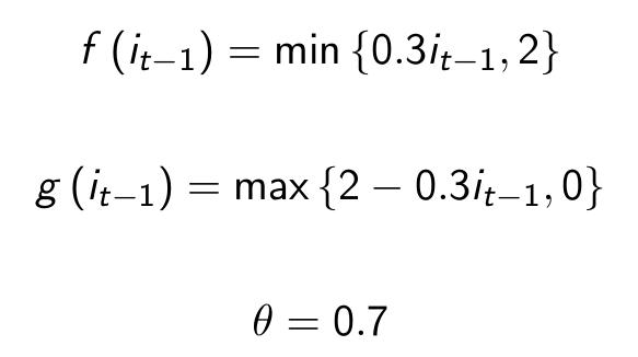
With the traditional rule in mind, I now propose an alternative that I call the Rate Dependent Taylor Rule. In this rule, set the instantaneous target (v) at

For some functions f and g that are weakly increasing and decreasing in the interest rate, respectively. Then set the actual rate as a weighted average of the interest rate last period and the current instantaneous target

For some θ between 0 and 1.

Therefore, a particular specification could be:

These response coefficients are plotted in the following chart. Observe that at the black line when the interest rate is 5, the two Rate Dependent coefficients match the traditional Taylor Rule.

There are three key design features of this specification.

First, the values of these coefficients are fixed in the range between 0 and 2. The logic behind this is to prevent excessive volatility in the interest rate. With these bounds, we also have justification for the slopes of 0.3. Recall that for the original rule, the coefficient on inflation was fixed at 1.5 and the coefficient on the output gap was fixed at 0.5. The modified rule takes on these values only if the interest rate is 5, the historical average of the federal funds rate. Therefore, the modified rule can both be more hawkish and more dovish than the original Taylor rule, contingent on economic conditions. This way, the modified Taylor rule can emulate the magnitude and volatility of the old Taylor rule, but also provide additional flexibility.

Second, when the interest rate is below 3.3, the example above actually violates the Taylor principle. This is no accident. Recall that the logic of the Taylor principle was to allow the central bank to keep a lid on inflation by ensuring that the real rate rises in response to inflation. But if interest rates are already at the low level of 2%, we actually want to encourage inflation so that the nominal rate can stay at the 5% level. Intuitively, this strengthens the negative feedback loop that keeps the nominal interest rate around 5%, giving the central bank more room to operate. 

Third, the interest rate is highly persistent. This is an issue discussed at length in Woodford's work "Optimal Monetary Policy Inertia", and there are two main justifications.

On one hand, excessive interest rate volatility can itself be harmful as agents spend more resources trying to avoid holding money. This is the argument for a Friedman rule for zero nominal interest rates, and although the argument is not as strong in the case, the logic still applies. High nominal rates can be distortionary, and thus their variance should be limited.

Moreover, without persistence it is hard for central banks to signal commitment to future interest rate paths. Future policy would be more unpredictable. Because the rate can change dramatically in response to new conditions, the Fed would not have a framework for commitment. Because one of the key selling points of a Taylor rule is to help guide expectations, to have an instrument that responds too quickly to economic conditions weakens the expectations channel. Therefore, the instrument should be persistent. In my rule, I choose a value of 0.7, which is very close to the value of 0.65 cited by Woodford.

3. Historical Comparisons

This specification is first compared against the traditional Taylor Rule and actual federal funds rate during the Great Moderation and up to the current period. Note that this isn't really a policy simulation. In fact the parameters that are rate dependent look at the actual federal funds rate in the previous period, not the rate-dependent rate. Therefore, this version gives a better picture of how the policy would give advice at each moment in time. In the future, I intend to further investigate the dynamics.

In the top panel are the various interest rates and rules. The red line is the actual effective Fed Funds rate, the gold line is the traditional Taylor Rule, and the green line is the Rate Dependent rule. The panel suggests that this interest rate rule actually fits monetary policy in the Great Moderation very well. In particular, comparing the traditional Taylor Rule with the Rate Dependent rule in the 2003-2007 period suggests that low interest rates may have been the justification for the downward deviation in the Taylor Rule.

The bottom panel shows a running time series with the coefficients in front of inflation (blue) and output gaps (magenta) changing over time. This shows that although the traditional Taylor Rule matches the policy advice of the Rate Dependent rule for the second half of the 1990's, in general they do not always correspond.

Another historical period of interest is the 1970's and 80's. In this time, inflation was far too high. Therefore, an effective rule should call for more hawkish policy. Indeed, the Rate Dependent rule does that. It would have called for interest rates in the 1970's and 1980's to be up to 10 percentage points higher than they actually were, and approximately five percent higher than what the traditional Taylor rule would have called for.

This is similar to what Evan Soltas noted about how a nominal GDP target would have called for tighter policy in the 70's. Even though the Rate Dependent rule would at times call for easier policy to stabilize output, it  is very hawkish when inflation is high. As such, it would still anchor inflation expectations with the promise of disciplined policy when inflation and the Fischer effect push up interest rates in the future.

4. Relationship with Forward Guidance, Nominal GDP Targeting, and a Virtual Fed Funds Rate

Although the Rate Dependent rule fits the historical data quite well, there is one large deviation. In the current environment, the rule says that the Fed should be easing. Hard. While the zero lower bound constrains the Fed from actually hitting the rate advocated by this rule, this does not mean the rule cannot help guide policy. In fact, the greatest appeal of the Rate Dependent rule at the current juncture would be its justification for forward guidance. If the large gap can't be closed with current short term rates, then perhaps it can be filled with future ones.

A Rate Dependent rule frames the current tightness in monetary policy by identifying a large deviations from a rule that fits the historical data. While this method may not be ideal, it shows how even the traditional framework of seeing monetary policy through instrument rules justifies aggressive easing at this juncture. 

Moreover, the theoretical reasoning behind the Rate Dependent rule is much more familiar for those who think in terms of Taylor Rules. Unlike a nominal aggregate target, the Rate Dependent rule is a concrete policy that can be implemented. It helps to assuage the concerns of John Taylor when he complains that an open ended nominal GDP target fails to give "quantitative operational guidance about what the central bank should do with the instruments." This way, the Rate Dependent rule helps to justify additional easing to a broader audience.

This alternate framing also gets around potential credibility issues nominal GDP targeting. This is not to say a nominal GDP target would  not be desirable but a 2012 Dallas Fed paper did bring up some credibility issues with such a target.  Evan Koenig, the vice president of the Dallas Fed, pointed out that the Fed does not have a good record of stabilizing nominal GDP growth. A graph from the paper is reproduced below. 

However, the historical comparisons above clearly show that the Rate Dependent rule is a good description of historical policy. Moreover the scatter plot below clearly shows that the Rate Dependent rule is also a good predictor of what a nominal GDP target would require. Therefore, the Fed can point to this rule and do a monetary two-step. While the Fed foxtrots into a more enlightened nominal GDP target, it can still maintain and demonstrate its credibility to this new policy path by justifying it with the historical experience.

The Rate Dependent rule is also a close cousin of the virtual Federal Funds rate, as advocated by my colleague Miles Kimball. In fact, the two proposals complement each other since the Rate Dependent rule provides a systematic approach for determining the virtual rate. This way, the Fed doesn't just ease when it "feels that monetary policy should be more expansionary." It would ease when it could point to the rule and say that it must.

5. Concluding Remarks

Of course, there is much work yet to be done. The above analysis is very descriptive and requires more formal modeling. In an upcoming post, I intend to discuss more about dynamics and the persistence of this rule. Doing more case study analyses of the rule in historical contexts would also be useful.

Much of the recent push for nominal GDP targets has neglected rules for the instrument. This omission runs the danger of confusion over the steps that need to be taken when a "whatever it takes" policy is declared. The Rate Dependent rule cuts through that confusion. It combines the rule based approach characteristic of traditional Taylor Rules with the recognition that the costs of inflation or output gaps can depend on the interest rate. In bridging various intellectual cousins, this policy forms a stronger basis for monetary easing now, while also committing to smart hawkishness later.

When the Zero Bound Didn't Bind

The zero lower bound didn't always bind. For three months after Lehman's collapse on September 15, 2008, the federal funds rate stayed above zero. In this period of time, the Fed managed to provide extensive dollar swaps for foreign central banks, institute a policy of interest on excess reserves, and kick off the first round of Quantitative Easing with $700 billion dollars of agency mortgage backed securities. Finally, on December 15, 2008, the Fed decided to lower the target federal funds rate to zero.

It is important to remember the sequence of these events. It is easy to think that the downward pressure on interest rates was the inevitable consequence of financial troubles. Yet the top graphic clearly contradicts this. Each of the dotted lines represents a FOMC meeting, and each of these meetings was an opportunity for monetary policy to fight back against the collapsing economy. The Fed's sluggishness to act is even more peculiar given that there were already serious concerns about economic distress in late 2007. As, the decision to wait three months to lower interest rates to zero was a conscious one, and one that helped to precipitate the single largest quarterly drop in nominal GDP in postwar history. The chaos in the markets did not cause monetary policy to lose control. Rather, the Fed's own monetary policy errors forced it up against the zero lower bound.

This is not to say those mistakes were purposeful. But in the high stakes game of central banking, even benign neglect can be dangerous. These failures in the last three months of 2008 can teach us many lessons about what should be done for future monetary policy. Only this way can we be more sure that careless mistakes won't jeopardize the future path of monetary policy.

One of the first steps would be to switch to a nominal GDP target. This would have two primary effects.

First, while this by itself is not a concrete instrument, it would be an important step in giving policy makers more freedom in responding to crises. Our current focus on inflation can cause particularly perverse outcomes when the economy comes under stress. During the September FOMC meeting right after the Lehman collapse and the Merill Lynch merger, in spite of the chaos in financial markets, the Fed chose to leave interest rates unchanged because of concerns about commodity price inflation. After such a long period of worrying economic conditions, the Fed choked because of a relative price change that was beyond the control of monetary policy to tame. A nominal GDP target would be robust to these kinds of shocks and better keep policy on track during the unfolding of a crisis.

Second, a nominal GDP target would also make policy after interest rates hit zero more credible.When the Fed is at the zero lower bound, one of the most important policy levers it has left is to adjust expectations of future interest rates. This is known as forward guidance, and is a consistent theme in the literature. In Krugman's original work on Japan's liquidity trap, he termed this kind of policy "credibly promising to be irresponsible". If this sounds peculiar, you are not alone. John Cochrane observes that

the key to stimulus when interest rates are zero is for the Fed to commit to keeping interest rates low, lower than than we and the Fed know it will want them to be when the time comes.

As a result, the Fed has a hard time committing to its forward guidance because it will want to renege in the future. However, if there were a nominal GDP target, this would remove the pressure to renege. In a sense, declaring a nominal GDP target changes perceptions of what the Fed wants.  By making policy systematic, and not discretionary, we can actually shape expectations and make the current policies of forward guidance and quantitative easing that much more effective.

For Sussing Out Whether Debt Affects Future Growth, the Key is Carefully Taking into Account Past Growth

On Miles' website we have a companion post to the previous post on an instrumental variables analysis of the RR dataset. In the companion post, we walk through more of the regressions and illustrate how controlling for past growth can erase almost any effect of debt on future growth. The core conclusion?

The two of us could not find even a shred of evidence in the Reinhart and Rogoff data for a negative effect of government debt on growth for either growth either in the short run (the next five years) or in the long run (as indicated by growth from five to ten years later).

Even though the estimated slopes are still small, we also discuss why this difference -- between small negative and small positive numbers -- matters for policy. For more, be sure to read the full post here.

Data Release

The data and code used in the Quartz column with Professor Kimball can be found on the data page here.

Instrumental Tools for Debt and Growth

A Joint Post by Miles Kimball and Yichuan Wang

In a recent Quartz column, we found that high levels of debt do not appear to affect future rates of growth. In the Reinhart and Rogoff (henceforth RR) data set on debt and growth for a group of 20 advanced economies in the post WW-II period, high levels of debt to GDP did not predict lower levels of growth 5 to 10 years in the future. Notably, after controlling for various intervals of past growth, we found that there was a mild positive correlation between debt to GDP and future GDP growth.

In a companion post, we address some of the time window issues with some plots how adjusting for past growth can reverse any observed negative correlation between debt and future growth. In this post, we want to address the possibility that future growth can lead to high debt, and explain our use of instrumental variables to control for this possibility.

One major possibility for this relationship is that policy makers are forward looking, and base their decisions on whether to have high or low debt based on their expectations of future events. For example, if policy makers know that a recession is coming, they may increase deficit spending to mitigate the upcoming negative shock to growth. Even though debt may have increased growth, this would have been observed as lower growth following high debt.On the other hand, perhaps expectations of high future growth make policy makers believe that the government can afford to increase debt right now. Even if debt had a negative effect on growth, the data would show a rapid rise in GDP growth following the increase in debt.

Apart from government tax and spending decisions informed by forecasts of future growth, there are other mechanical relationships between debt and growth that are not what one should be looking for when asking whether debt has a negative effect on growth. For example a war can increase debt, but the ramp of the war makes growth high then and predictably lower after the ramp up is done and predictably lower still when the war winds down. So there is an increase in debt coupled with predictions for GDP growth different from non-war situations. None of this has to do with debt itself causing a different growth rate, so we would like to abstract from it. 

To do so, we need to extract the part of the debt to GDP statistic that is based on whether the country runs a long term high debt policy, and to ignore the high debt that arises because of changes in expected future outcomes or because of relatively mechanical short-run aggregate demand effects of government purchases as a component of GDP. Econometrically, this approach is called instrumental variables, and would involve using a set of variables, called instruments, that are uncorrelated with future outcomes to predict current debt.

Since we are considering future outcomes, a natural choice for instrument would be the lagged value of the debt to GDP ratio. As can be seen below, debt to GDP does not jump around very much. If debt is high today, it likely will also be high tomorrow. Thus lagged debt can predict future debt. Also, since economic growth is notoriously difficult to forecast, the lagged debt variable should no longer reflect expectations about future economic growth.   
By using lagged debt and growth as instruments, we isolate the part of current debt that reflects debt from a long term high debt policy, and not by short run forecasts or other mechanical pressures. We plot the resulting slopes on debt to GDP in the charts below, for both future growth in years 0-5 and for future years 5-10. For the raw data and computations, consult the public dropbox folder.


From these graphs, we can make some observations.

First, almost all the coefficients, across all the different lags and fixed effects, are positive. Since these results are small, we should not put too much weight on statistical significance. However, it should be noted that the plain results, OLS and IV, for both growth periods are all statistically significant at at least the 95% confidence level, and the IV estimates for the 5-10 year period in particular are significant at the 99% confidence level.

The one negative estimate, OLS estimate with country fixed effects, has a standard error with absolute size twice as large as the actual slope estimate.Moreover, country fixed effects are difficult to interpret because they pivot the analysis from looking at high debt versus low debt countries towards analyzing a country's indebtedness relative to its long run average.

These results are striking considering therobustness with which Reinhart and Rogoff present the argument thatdebt causes low growth in their 2012 JEP article.Yet instead of finding a weaker negative correlation, aftercontrolling for past growth, we find that the estimated relationship between current debt and future growth is weakly positive instead.

Second, when taking out year fixed effects, there is almost no effect of debt and future . Econometrically, year fixed effects takes out the average debt levelin every year, which leaves us analyzing whether being more heavilyindebted relative to a country's peers in that year has an additional effect on growth. Because this component isconsistently smaller than the regular IV coefficient, this suggests,for the advanced countries in the sample, it's absolute, not relative, debt that matters.

This should be no surprise. As most recently articulated in RR's open letter to Paul Krugman, much of the argument against high debt levels relies on a fear that a heavily indebted country becomes “suddenly unable to borrow from international capital markets because its public and/or private debts that are a contingent public liability are deemed unsustainable.” The credit crunch stifles growth and governments are forced to engage in self-destructive cutbacks just in order to pay the bills. At its core, this is a story about whether the government can pay back the liabilities. But whether or not liabilities are sustainable should depend on the absolute size of the liabilities, not just whether the liabilities are large relative to their peers.

Now,our conclusion is not without limitations. As Paul Andrew notes,the RR data set used focuses on “20 or so of the most healthy economies the world has ever seen,” thus potentially adding a high level of selection bias.

Additionally, we have restricted ourselves to the RR data set of advanced countries in the post WW-II period. The 2012 Reinhart and Rogoff paper considered episodes of debt overhangs from the 1800's, and thus the results are likely very different. However, it is likely that prewar government policies, such the gold standard and the lack of independent monetary authorities, contributed to the pain of debt crises. Thus our timescale does not detract from the implication that debt has a limited effect on future growth in modern advanced economies.

In their New York Times response to Herndon et. al., Reinhart and Rogoff “reiterate that the frontier question for research is the issue of causality”. And at this frontier, our Quartz column, Dube's work on varying regression time frames, and these companion posts all suggest that causality from debt to growth is much smaller than previously thought.