Monetary Axioms II: The Movement of Expectations with Respect to Shocks

Pity that these concepts are "counter-intuitive"

I quite enjoyed my last definition/proposition/lemma/theorem post, and although many of the statements were axiomatic or self-evident, they led me to an interesting realization about current nominal GDP growth, credible monetary policy, expected future nominal GDP growth,  and interest rates.

While we often talk about nominal GDP gaps, I would like to start the drawing and theorem process by looking at graphs of nominal GDP growth. Below is a graph of log nominal GDP (right) and continuously compounded annual rates of nominal GDP growth (left), both reported quarterly.

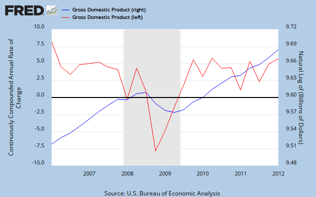
In terms of calculus, nominal GDP is the level of the variable, whereas the growth rate is the instantaneous derivative. Note that although the level falls significantly from its previous trend, the growth rate returns to a value that's similar to its pre-crisis trend. However, even a temporary shock in the growth rate can cause a permanent fall in the level if there is not a restoring amount of growth after the shock.

By looking at the growth rate, we can determine the size of the output gap by integrating, or looking at the area. The integral of the growth rate minus the integral of the trend rate is the size of the output gap, as shown in the stylized diagram below in which trend growth is simplified, without loss of generality, to 0%.

From this, we can see that growth rate targeting can leave large gaps in the actual level. Since the central bank moves the growth rate to the precrisis rate of 0, it leaves the output gap. This can be corrected by level targeting, which tries to get the level of the variable back to pre-shock trend growth. This entails a period of growth above 0 to balance the output gap. How much higher? For how long? Mathematically, the integral of the curve over this time period should be zero. Graphically, it means that the higher rate must be sustained until the blue area (positive growth) minus the red area (negative growth) equals zero. This means the red and blue areas should be the same.

By the calculus definition, the average of a function over an interval is the integral of the function over the interval divided by the size of the interval. In this context, it means that the average growth of nominal GDP over the entire period is zero, the original trend growth rate. We have therefore successfully targeted the level of nominal GDP.

To start looking at credible nominal GDP targeting in this framework, let's define some time lengths:

Definition: The crisis time (c) is the period of time starting with the formation of the output gap to the conclusion of the policy response.

Definition: The expectation horizon (e) is the period of time that economic agents forecast and use to determine their expectation of future nominal GDP growth.

For the discussion below, I will assume that before the negative shock, economic agents were unable to forecast the shock; this is the reason why the credible level targeting didn't solve the shock before it happened. However, once the shock takes place, economic agents are fully aware of the time path of nominal GDP growth that occurs as a result of the shock and policy response. Importantly, agents know that the central bank is committed to level targeting, and that this declaration is credible. This means that the private sector knows the areas, red and blue, will be the same in the end. 

In reality, these would all be expectations. But I will accept the rational expectations hypothesis that expectations match the reality for the purposes of this benchmark model.

Let us start with a special case, in which the expectation horizon is equal to the crisis time, as pictured below.

What is the expectation of economic agents of average nominal GDP growth over the expectation horizon at time to? As both areas are equal to each other, the integral over the expectation horizon is zero, so average expected nominal GDP growth is also zero. No surprise there. But what about at some time in the middle of the output gap, say at tm? The integral is then positive! The integral is represented in the graph below by the blue area minus the pink area (note that trend growth is zero after the policy response). As you can see, the blue area is larger, making the integral positive. Because  expected average nominal GDP growth is the interval divided by the expectation horizon e, the expectation of nominal GDP growth also becomes positive.

As a result, if monetary policy is perceived as credible enough to solve the shock in the same interval as the expectation horizon, a current negative nominal GDP shock manifests itself in increased expectations of nominal GDP growth over the expectation horizon. The graph would look something like this:

A similar result is obtained if the expectation horizon is greater than the crisis time (e>c). Just move to+e to the right, and both the nominal GDP growth and the expectation curves return to zero at to+c.

This result might seem puzzling, as this hardly seems like what happens in real life. To get to "real life" monetary policy, imagine a world with highly inertial policy, such that the crisis period is longer as policy takes more time to respond and the output gap lasts longer as a result. We would be in a world such as that below:

From here, the growth expectation at time to is the value of the pink area divided by e. Although e is chosen such that to+e is to the left of the policy response, as long as e is less than c, the expectation will start out negative. The expectation curve moves forward in a different manner compared to the e=c case. The expectation does become positive when the [to, to+e] interval only covers the blue portion. As a result, the expectation over the period looks like this:

Note that the exact curvature is dependent on the function for the shock and the expectation horizon. But it should be noted that the max/min of the expectation curve should not go past the max/min of the actual path for nominal GDP growth.

Flipping the directions of the output gap and policy response gives us the result for a positive aggregate demand shock, and they are, predictably, the opposites of the ones we obtain for a negative shock.

This long and winding road then allows us to conclude the following:

Theorem: Given a monetary regime that has a credible nominal GDP level targeting policy:

1. If the crisis period is greater than the expectation horizon, expectations of nominal GDP will be procyclical to current nominal GDP growth.
2. If the crisis period is less than or equal to the expectation horizon, expectations of nominal GDP with be countercyclical to current nominal GDP growth.

This gives us a yardstick to judge if a monetary policy is credibly level targeting for a variety of expectation horizons. Most importantly, if treasuries of varying maturities are correlated with expected nominal GDP growth over the treasuries' time periods, then we can look at the movement of treasuries to judge forecasts of crisis lengths in credible level targeting regimes. The treasuries with yields that rise have maturities beyond the crisis period, while the treasuries with yields that fall have maturities within the crisis period. This also solves the data problem, as we now can find out the market's observations about current GDP growth by looking at its expectations of future NGDP growth.

Although the model outlined above discusses level targeting, it can be extended to rate targeting as well. Think of rate targeting as a form of level targeting whose "policy response" is to hope a positive shock comes the other way in the future. In effect, rate targeting is level targeting with an extremely long crisis period. As a result, shocks to nominal GDP growth in a rate targeting regime almost fall into the first case of the theorem for most expectation horizons. By this theory, current yields on long term treasuries betray a very negative outlook on future nominal GDP.


As this model uses interest rates as a way of gauging expectations, they work the best when interest rates are allowed to float and communicate information. If these interest rates were targeted, the central bank would be suppressing a key source of information. This is another advantage of a NGDP futures level targeting regime versus an interest targeting regime. High interest rates won't be confused for "tight money" if the interest rate is determined by the market.


This post should remind us that Market Monetarism is a world of non-linear causality and counter-intuitive movements in both expectations and interest rates. Except they wouldn't be counter-intuitive and these arguments would be self evident if policy actually targeted the level of nominal GDP. Alas, the Fed does not. A great shame, for both both our learning of intuition and suffering in this nation.

Edit (7/13/2012): Fixed the grammar in the last three paragraphs, no substantive change in the message.